In many real life applications where we wish to evaluate a function, we are only able to define the relationship that the derivative of that function must satisfy. One example is the dynamics of a vehicle in which we wish to determine the velocity or acceleration, however the unknowns are specified only in terms of ordinary differential equations (ODEs) and initial conditions. In this note we wish to show one approach to the numerical solution of ODEs using MATLAB and the Classical fourth order Runge-Kutta method. This is a very personal approach and is somewhat different to that normally used, however I will try to justify it further on. The simplest non-trivial example that I could think of to develop this approach is that of the large angle pendulum
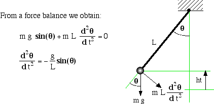
Consider a simple pendulum having length L, mass m and instantaneous angular displacement θ (theta [radians]), as shown below:
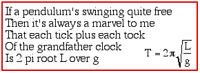
For small initial angles θ we make the assumption that sin(θ)=θ leading to the well known analytical solution:
(Refer: Top 150 Limericks)
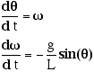
However for large angles θ we resort to a numerical method to solve the differential equation above. We first reduce the second order differential equation to a set of two first order differential equations by introducing ω (omega - angular velocity [radians/s]), leading to:
Fortunately we can always reduce a n-th order ODE into a n-vector set of first order ODEs. Thus we need only concentrate on developing numerical techniques for solving a vector set of first order ODEs. Processing vectors by computer simply requires looping sequentially through the indices of the vector, and MATLAB is particularly geared to this type of analysis. MATLAB provides five separate routines for solving ODEs of the form dy = f(x,y) where x is the independent variable and y and dy are the solution and derivative vectors. They are extremely simple to use, however they do not provide the versatility that I am looking for, including choosing the step size dx and overloading the y-vector. For example consider the case that we wish to determine the height (ht) of the pendulum mass as shown in the above diagram. This does not require a differential equation since the height is related to the angle θ as follows:
Consider now the practical aspects of writing a function for evaluating this set of derivatives. One problem is that vectors are usually assigned generic names such as y for the set of dependent variables and dy for their derivatives, however we would like to retain their identity in terms of θ (theta), ω (omega) and height. This makes the programs much more readable, and can be easily done by means of indices, as shown in the MATLAB function below:
function [y,dy] = dpend(t,y) % dpend.m - The pendulum differential equations % g [m/s^2] acceleration due to gravity % length [m] pendulum length % Izzi Urieli - Jan 21, 2002 (updated 12/08/07) global g length THETA = 1; % index of angle [radians] OMEGA = 2; % index of angular velocity [rads/sec] HEIGHT = 3; % index of pendulum mass height [m] dy(THETA) = y(OMEGA); dy(OMEGA) = -(g/length)*sin(y(THETA)); y(HEIGHT) = length*(1 - cos(y(THETA))); |
Notice the use of upper case characters for the indices as is the convention in programming, however all other variables (including the global variables) begin with a lower case letter. Notice also both y and dy are returned (instead of only dy as is normally done). This is because the y-vector has been "overloaded" with the height variable which is evaluated as a function of θ in this function. This option is not available in MATLAB using their conventional ODE solving routines, however I find that I need to use it extensively.
Consider now a typical main function for this case study:
% pend_rk4.m - Solve the large angle pendulum problem using rk4
% Izzi Urieli - December 8, 2007
clear all
THETA = 1; % index of angle [radians]
OMEGA = 2; % index of angular velocity [rads/sec]
HEIGHT = 3; % index of pendulum mass height [m]
global g length
g = 9.807; % [m/s/s} accel. due to gravity
length = input('Enter pendulum length [m]: ');
angle0 = input('Enter initial pendulum angle [degrees]: ');
period = 2*pi*sqrt(length/g);
fprintf('small angle period is %.3f seconds\n',period);
tfinal = 1.5*period;
%######################using rk4:
n = input('Enter the number of solution points: ');
dt = tfinal/(n - 1);
t = 0;
y(THETA) = angle0*pi/180; % initial pendulum angle [radians]
y(OMEGA) = 0;
y(HEIGHT) = length*(1 - cos(y(THETA))); % initial pend. height [m]
time(1) = t;
angle(1) = angle0;
height(1) = y(HEIGHT)*100; % cm (for scaling on the plot)
for i = 2:n
        [t, y, dy] = rk4('dpend',2,t,dt,y);
        time(i) = t;
        angle(i) = y(THETA)*180/pi;
    height(i) = y(HEIGHT)*100;
end
%##############################plotting:
plot(time,angle)
grid on
hold on
axis([0 tfinal -90 90])
x0 = [0,tfinal];
y0 = [0,0];
plot(x0,y0,'k-')
x1 = [period,period];
y1 = [-90,90];
plot(x1,y1,'r-')
plot(time,height, 'g-')
xlabel('time [seconds]')
ylabel('pendulum angle[degrees], height[cm] (green)')
title('pendulum angle and height vs time')
|
As with many MATLAB functions, this one is very short and mostly self-documenting. Notice that after specifying the system parameters we use the for loop to build the time, angle, and height arrays in order to plot them. The most interesting aspect of this program is the rk4 function call, to integrate one step dt of the differential equation set given in function dpend, as follows:
[t, y, dy] = rk4('dpend',2,t,dt,y);Thus the input arguments are the string constant representing the derivative function dpend, the number of differential equations in the set (2), the independent variable and increment (t,dt), and the dependent variable vector (y). The output arguments are the solution variables and derivatives [t,y,dy] integrated over one time step dt.
One of the most widely used of all the single step Runge-Kutta methods (which include the Euler and Modified Euler methods) is the so called 'Classical' fourth order method with Runge's coefficients. Being a fourth order method (equivalent in accuracy to including the first five terms of the Taylor series expansion of the solution) it requires four evaluations of the derivatives over each increment dx, denoted respectively by dy1, dy2, dy3, dy4. These are then weighted and summed in a very specific manner to obtain the final derivative dy, as follows:
function [x, y, dy] = rk4(deriv,n,x,dx,y)
% rk4.m - Classical fourth order Runge-Kutta method
%Integrates n first order differential equations
%dy(x,y) over interval x to x+dx
%Izzi Urieli - Jan 21, 2002
x0 = x;
y0 = y;
[y,dy1] = feval(deriv,x0,y);
for i = 1:n
        y(i) = y0(i) + 0.5*dx*dy1(i);
end
xm = x0 + 0.5*dx;
[y,dy2] = feval(deriv,xm,y);
for i = 1:n
        y(i) = y0(i) + 0.5*dx*dy2(i);
end
[y,dy3] = feval(deriv,xm,y);
for i = 1:n
        y(i) = y0(i) + dx*dy3(i);
end
x = x0 + dx;
[y,dy4] = feval(deriv,x,y);
for i = 1:n
        dy(i) = (dy1(i) + 2*(dy2(i) + dy3(i)) + dy4(i))/6;
        y(i) = y0(i) + dx*dy(i);
end
|
The most interesting aspect of this function is the use of the MATLAB function feval to evaluate the function argument which is passed as a string. This is a fundamental aspect of MATLAB programming, and understanding this is essential to developing MATLAB programs.
The three MATLAB function mfiles shown above pend_rk4.m, dpend.m, and rk4.m can be downloaded and executed as required.
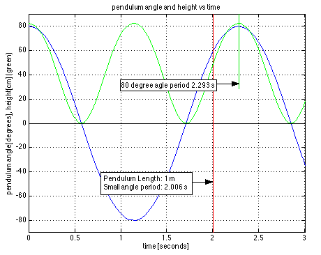
The plotting capabilities of MATLAB are extremely simple to use and very versatile. A typical output plot (with labels added) for this pendulum case study follows:
Notice that the small angle period is about 2..0 s, however at 80 degrees the period is seen to be signicantly increased (2.293 s). This could only have been determined by numerically solving the nonlinear differential equation set. Notice also the height plot which was added in order to illustrate the method of "overloading" the y-vector.
I asked Dr. John Cotton (our MATLAB guru) to comment on this approach - his response was:
"Matlab a few years back transitioned to using
function handles in place of feval (which may be phased out in the
future).
If for some reason you had a nasty function or just
wanted to use the Matlab solvers (ODExxx) you could still do what you
are doing here. The options allow controlling step sizes (or error
tolerances) for the canned solvers. (This is beyond what many
students are shown or educated to use however, which I tend to drone
on about to them.) There are ways of getting the heights out as a
separate variable using extended argument lists so you don't need to
overload the y vector, although I would have calculated the height
vector from the angles right before plotting in your main function.
(Then again "toMAYto, toMAHto".)"
Oh well! Obviously the Large Angle Pendulum problem presented above is a contrived example. This technical note serves mainly as an introduction to solving significantly more complex problems, such as the Adiabatic Analysis of Stirling Cycle Machines - (Then again "poTAYto, poTAHto".)