In many real life applications where we wish to evaluate a function, we are only able to define the relationship that the derivative of that function must satisfy. One example is the dynamics of a vehicle in which we wish to determine the velocity or acceleration, however the unknowns are specified only in terms of ordinary differential equations (ODEs) and initial conditions. In this note we wish to present an example of determining and solving the ODEs of an electric scooter using a permanent magnet dc electric motor. In particular we wish to evaluate the match between the motor and the scooter. We will use the popular built in MATLAB routine ode45 which uses a fourth and fifth order Runge-Kutta method.
Consider a typical scooter such as the "zappy2" made by Zero Air Pollution (ZAP no longer in production.)
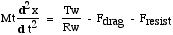
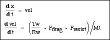
This scooter uses a simple permanent magnet dc motor running off a twelve volt battery. It does not have a throttle and uses a simple on/off switch for electrical assist.We wish to determine the scooter performance - acceleration from a stationary position until it reaches steady state speed. The equations of motion are relatively simple to derive - from Newtons Second Law the total mass times acceleration equals the applied force at the wheel minus the wind drag and resisting forces. Thus
where: x is the distance travelled [m]
Mt is the total mass (scooter + rider) [assume 100kg]
Tw is the torque applied at the wheel [Nm]
Rw is the radius of the wheel [assume 10cm]
Fdrag is the force due to wind resistance [N]
Fresist is the resistance force due to Rolling resistane and uphill slope [N]
also:
 where: ρ is the air density [assume 1.18 kg/m3]
CdA is the Drag Coefficient times the frontal area [assume 0.6 m2 for the scooter]
and
where: ρ is the air density [assume 1.18 kg/m3]
CdA is the Drag Coefficient times the frontal area [assume 0.6 m2 for the scooter]
and
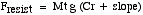 where: g is the acceleration due to gravity [9.807 m/s2]
Cr is the Coeffient of Rolling resistance (assume 0.01 for rubber tyre on tarmac]
slope is the elevation divided by the distance [assume zero]
where: g is the acceleration due to gravity [9.807 m/s2]
Cr is the Coeffient of Rolling resistance (assume 0.01 for rubber tyre on tarmac]
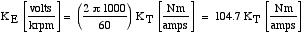
slope is the elevation divided by the distance [assume zero]The question is how to determine the torque applied at the wheel Tw. A basic characteristic of a PM dc electric motor is that its torque produced is linearly proportional to its current drawn, and similarly the back emf produced is proportional to the rotational speed, as shown in the following diagram:
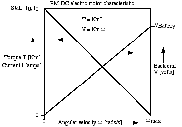
Thus    T = KT I
       V = KT ω
     where:    T is the motor torque [Nm]
              I is the motor current [amps]
              V is the back emf [volts]
              ω is the angular speed [rads/s]
              KT is the torque constant [Nm/amps]
Note that the back emf constant KE is often specified having units [volts/krpm], however this value can be restated in terms of KT as follows:
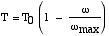
From the diagram above the motor torque is determined as a function of angular velocity ω as follows:
Note from the diagram that the maximum speed condition (ωmax) occurs at zero torque, when the back emf reaches the battery voltage, and the maximum torque T0 and maximum current I0 occur at stall. Furthermore the motor winding resistance Ω [ohms] can be measured under stall conditions:
VBattery = I0 Ω
Substituting these conditions into the torque equation above and simplifying:
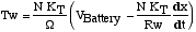
The motor torque is transferred to the scooter wheel through the transmission gear ratio, thus:
        where:   N is the transmission gear ratio
             ωw is the anular velocity of the wheel [rads/s]
             Tw is the torque applied at the wheel [Nm]
Finally, substituting all of the above and simplifying, we obtain the torque applied at the wheel as follows:
The various motor parameters discussed above - KT, Ω, ωmax, T0, I0, should all be available from the motor manufacturer, together with curves of power and efficiency. Thus for example in order to continue with this simulation I searched the web and came up with a motor from Minnesota Electric Technologies. I downloaded the specs of a motor that I decided to evaluate - model 3A-ww121126 from their Series 32 models and used this data in the simulation program below. (Unfortunately MET have removed all technical data and downloads from their current website)
I did run into a problem. Dr Foley mentioned to me that one should always do a steady state check from the graphs by matching the loads and not simply rely on the computer solutions of differential equations. I said "of course!" however when I checked the results I found that at the steady state speed of the scooter the motor rpm was higher than the published experimental no load rpm. This occurs because at no load the motor is drawing current and overcoming its own friction, hence the back emf constant is slightly higher than the torque constant KT. I decided to define a motor back emf constant KE as follows:
     KE = VBattery/ωno-load
        where:  ωno-load is the no load angular velocity [rads/s]
The data sheet from our chosen evaluation model does provide this information, however it can be easily evaluated by testing the motor under no load conditions. The modified equation of torque applied at the wheel now becomes:
Gathering the relevant equations from above, we have:
In order to solve the above second order differential equation, we need to rewrite it as a set of two first order differential equations. This is done by defining a new variable vel (velocity) leading to the following set:
Fortunately we can always reduce a n-th order ODE into a n-vector set of first order ODEs. Thus we need only concentrate on developing numerical techniques for solving first order ODEs. Processing vectors by computer simply requires looping sequentially through the indices of the vector, and MATLAB is particularly geared to this type of analysis.
Consider now the practical aspects of writing a function for evaluating this set of derivatives. One problem is that vectors are usually assigned generic names such as 'y' for the set of dependent variables and 'ydot' for their derivatives, however we would like to retain their identity in terms of velocity and distance. This can be done by means of indices, as shown in the MATLAB m-function below:
function ydot = dscoot(t,y) %dscoot.m - electric scooter differential equations of motion % Dr.Iz (Urieli) 02/14/04 (modified 2/16/04 to include ke) % y(DIS) = distance covered (m) % y(VEL) = velocity (m/s) DIS = 1; VEL = 2; % scooter basic parameters: mt = 100.0; % total mass of scooter + rider (kg) rw = 0.1; % wheel radius (m) % MET 3A-ww121126 motor specs: winding = 0.0965; % resistance (ohms) kt = 0.0334; % torque constant (Nm/A) ke = 0.0388; % back emf (volts/(rads/s)) (from no-load rpm) % wheel/motor transmission ratio: n = 8; % wheel_torque / motor_torque % battery voltage: vbat = 12; % (volts) % applied torque at rear wheel tw: tw = (n*kt/winding)*(vbat - ke*n*y(VEL)/rw); % current drain (how can we display this?) im = tw/(n*kt); % resistive forces: drag, slope, rolling resistance cda = 0.6; % coef. of drag * frontal area (m^2) density = 1.18; % air density (kg/m^3) drag = cda*density*y(VEL).^2/2; cr = 0.01; % coefficient of rolling resistance slope = 0.0; % no slope at this stage g = 9.807; % gravity (m/s^2) resist = mt*g*(cr + slope); ydot(DIS) = y(VEL); % velocity ydot(VEL) = (tw/rw - (drag + resist))/mt; % acceleration ydot = [ydot(DIS); ydot(VEL)]; % must be column vector |
Notice the use of upper case characters for the
vector indices as is the convention in MATLAB.
Consider now a typical main function for this case study:
%scoot.m - electric scooter simulation demo
% Dr.Iz (Urieli) 02/14/04
tspan = [0,10]; % time span to integrate over (10 seconds)
y0 = [0;0]; % initial [position;velocity] (starting from stop)
[t,y] = ode45('dscoot',tspan,y0);
size(t) % how many steps were evaluated? - simply curious
velo = y(:,2).*9/4; % velocity (mph) [9mph = 4m/s]
plot(t,velo,'k')
grid on
xlabel('elapsed time (s)')
ylabel('velocity (mph)')
title('dynamic simulation of electric scooter')
|
As with many MATLAB m-functions, this one is very
short and mostly self-documenting. The resulting plot follows.
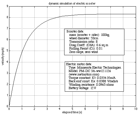
Thus we see that with the motor chosen we will reach steady state of around 8.2 mph within 10 seconds. It would not have been possible to obtain this information without solving the differential equations numerically.
Notice that I have doctored the plot somewhat by adding all the relevant parameters of the simulation. This should always be done. Nothing is more frustrating than trying to understand a plot or diagram in which the relevant information is missing.
The above simulation is for the Zappy, that does not
have a throttle and uses a simple on/off switch for electrical
assist. In the more general case we would have a throttle and
possibly a reversing capability, leading to the need for a
controller. An interesting tutorial website is that of the English
company 4QD
which specialises in controllers. They also have a
tutorial website with limited free public access 4QD-TEC
(The Electronics Club)