MATLAB Teaching Tools and Utilities Developed by Prof. Tingyue Gu

University instructors may request free MATLAB source codes for the following software (excluding utilities) by e-mailing gu@ohio.edu. Other far more advanced applications are available upon request. For custom made applications, please inquire. Standalone windows executable versions that do not require MATLAB to run are available upon request. MATLAB Version 7.x or above is required. Each MATLAB GUI (Graphical User Interface) application has two component, one it the m-file, another the .fig file containing the GUI face and initial settings.

Example 1. Nonlinear Algebraic Equation System Solver using MATLAB's folve

This software can be used to teach the importance of fsolve initial values. It shows the residuals to let user check the quality of the results. A warning is given if fsolve's Exitflag is not equal to one. (Example: Add x4^2-100 and initial guess 0 to the default equation set.) This solver can solve up to 99 nonlinear algebraic equations simultaneously. Equations can be entered on the screen or supplied in a .txt file. A student can use the File menu to generate a simple non-GUI m-file to study its contents. The simple m-file can be run in the MATLAB command console to solve the same problem without GUI. This MATLAB GUI application can also be used as a tutorial to teach GUI designs and string handling. MATLAB Version 7.x or above is required. Download this software here. This application can be compiled to make a standalone application with MATLAB runtime library files. MATLAB R14 started to allow the "eval" function to be used in Compiler Version 4.0.

Example 2: Numerical ODE Solver using Euler or Runge-Kutta Method for math classes

This application can be used to demonstrate convergence of an ODE's numerical solution by changing the number of t nodes. It can also be used to compare the Euler method's accuracy with that of Runge-Kutta method's. Its source code can be used as a tutorial to teach a simple MATLAB GUI design. Download a p-code package here. You can run the p-code just as an m-file, except that p-code is binary. Instructors can request source code m-file. The source code cannot be requested by students because instructors often ask students to write Euler and Runge-Kutta codes as assignments. However, a version that uses MATLAB ode45 and ode15s can be downloaded here. 

Example 3. Graphical MATLAB software to solve two ODEs numerically

This application allows the user to solve very stiff nonlinear problems when MATLAB's ode15s is used instead of ode45 or Runge-Kutta. When the answers are plotted in an external figure window, the figure can be saved or copied neatly to Microsoft WORD. Download a p-code package here. You can run the p-code just as an m-file, except that p-code is binary. The source code is available to instructors, and students (with Runge-Kutta code lines removed) upon request. MATLAB Version 7.x or above is required. The source code cannot be requested by students because instructors often ask students to write Runge-Kutta code as an assignment. However, a version that uses MATLAB ode45 and ode15s only can be downloaded here. 

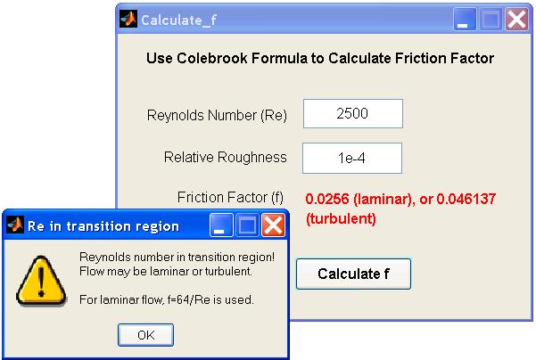
Example 4. Graphical MATLAB software for friction factor calculation in Fluid Mechanics

This application eliminates the need to use the Moody chart for friction factors. Colebrook formula is used for turbulent flow, and f=64/Re for laminar flow. This simple MATLAB GUI application can also be used to teach simple GUI designs. MATLAB Version 7.x or above is required. Download this software (source code) here.

MATLAB Utilities and Tips 

1. MfigExtract (a utility to extract x-y data in MATLAB figure files) 
In a project, it is convenient to save data as MATLAB figures with labels instead of dull data array files. What if you lose the data array files? Relax! MATLAB figures have x-y data sets embedded inside. Here is a user-friendly free utility coded by Dr. Gu to extract x-y data series into an Excel file from MATALB figure (.fig) files. MATLAB R17 (Version 7.x) or higher is needed to run this program. 

2. LEDbar (an LED style embedded progress bar for time-consuming loops)
It gives a program a professional look if you add a progress bar (also known as wait bar) to indicate the percentage progress or time for a lengthy loop. You may also wish to add an ABORT button. MATLAB has a built-in waitbar function. A waitbar window pops out for it. Its default position is at the center of the screen. You cannot easily change the position. An embedded progress bar is more desirable sometimes. I tried some of the methods out there, but they cause flickering of the main GUI screen because they use an embedded figure on the main GUI screen. Figure updating causes flickering even with 'DoubleBuffer' is set to 'on' value. In LEDbar, 10 colored text fields are created in 'guide' to act as 10 LED lights. Each of the 10 LEDs is turned on sequentially with each 10% progress. LEDbar can be dragged to any part of the main GUI screen by beginners. See screen shot below. Download examples and check out M-file source codes here. LEDbar is freeware.

3. How to embed logo (or background image) in GUI layout?
Create a GUI (say test.m with test.fig). Add Axes. Properties: Units=pixels, Position: Width=192, heigh=228 (assume logo.bmp is 192x228 pixels in size). Right click to select Create_Fcn. In the m-file, under the Create_Fcn section for the newly created Axes, add lines logoimage=imread('logo.bmp');  image(logoimage); axis off;

Here is the funny side of this. You can run test.m in MATLAB now. However, you need test.m, test.fig and logo.bmp all in the same directory. After you run test.m at least once, open the GUI and do something (such as slightly moving your logo position). Now, save your GUI. You will see that your test.fig file size has been increased. This means logo.bmp has been embedded inside test.fig. You can delete logo.bmp file and delete the lines corresponding to the Axes Create_Fcn. (This undocumented method has been tested in Versions R13 and R14.) You may ask me, why don't you use the newest MATLAB version? Well, its runtime library package is over 100 MB for the compiled .exe deployment. R13 compiler needs only 8 MB!

4. How to change background color for an edit field in GUI layout?
Mathworks says that you cannot change the default white color for an Edit field in R13 and R14 For a Text field, there is no problem. Go figure! I found a way to work around this. First create a Text field. Then, change it to Edit field by using Property Inspector's Style menu. By the way, the default MATLAB GUI color scheme is Hue=34, Sat=83, Lum=213; Red=236, Green=233, Blue=216. If you still have problems, search for 'white' and replace it with 'gray' for the field that you want change its background in the main m-file. 

5. Utility for internet authentication of license 
This is good for shareware or evaluation software. You can code each copy of your software with a key string that has to be matched with a key string in a web file on your server. The copy of software can be enabled or disabled anytime remotely by setting or removing the key in the web file. You can track how many time the license file has been accessed and from which IPs by configure your web server settings. You can also set IP or IP ranges so the software can only be used by certain machines. Universities typically use Class B IP numbers. You can set the IP range and the copy of software can no longer be used at a commercial site. E-mail me to get this simple utility's source code m-file. 

6. "AddFigureMenus Version 1" utility for GUI embedded plots or plots generated by standalone MATLAB applications 
If you open a figure (with plotted lines/curves) in the MATLAB command console, the figure can be manipulated in various ways such as changing title, label, legend, line style and copying to clipboard for pasting to Microsoft WORD and Excel, etc. This is not true for some other situations. Case 1. Suppose you run your GUI application in the MATLAB command console. If you embed a plot inside a GUI layout, lines in the figure cannot be edited unlike in a plot in a separate figure window. Case 2. Suppose you run a compiled standalone application. It is known to developers that there is only a File menu. The File menu can only be used to save or print a figure. It cannot be used to manipulate the figure in any way except zooming and rotating. It cannot be even copied to clipboard for pasting. AddFigureMenus was created by me to add extra menu items so that a figure can be manipulated directly once a figure is created by a standalone application without using MATLAB command console. The AddFigureMenus functions (including AddEditMenu, AddEditMenu4subplot and AddContextMenu) are easy to use. Just call them as needed after each plot. Figures with subplots are OK. Just click on a subplot before choosing an Edit menu option. See the example below. They provide many useful ways to manipulate a figure. X-Y values at any point on a line can be displayed by right licking the mouse button. This software is compatible with Compiler Version 3 (R13) and above. Because of likely commercial applications, sources codes are not freely available. Download p-code files here. Call the p-code functions just like calling m-functions without changing anything in your main M-file. Examples are included. M-files calling the p-codes can be compiled using R14 or above. 

function test_main
plot ([1 2 3],[1 3 5],'Color','r','LineWidth',2)
title('x-y figure'); xlabel('x (m^2)'); ylabel('y (Pa)')
text(1.515,2,'\bullet\leftarrow\alpha_1= \pi')
AddEditMenu(gcf); 
hold
plot([1 2 3],[1 2 3],'LineWidth',2); legend('curve 1','curve 2')
AddContextMenu(gcf) %add context menu to all lines, new and old