function plotmass
% Kyle Wilson 10-2-02
% Stirling Cycle Machine Analysis ME 589
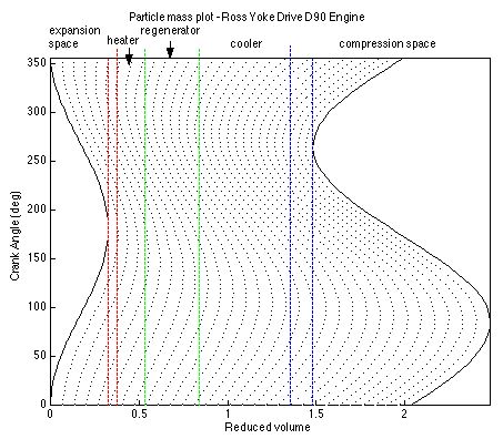
% Particle Trajectory Map
% Equations from Organ's "'Natural' coordinates for analysis of the practical
% Stirling cycle" and Oegik  Soegihardjo's 1993 project on the same topic
% Modified by Israel Urieli (11/27/2010) to obtain correct phase advance
% angle alpha subsequent to error determined by Zack Alexy (March 2010)

% Global values from define program
global vclc vcle % compression,expansion clearance vols [m^3]
global vswc vswe % compression, expansion swept volumes [m^3]
global alpha % phase angle advance of expansion space [radians]
global vk % cooler void volume [m^3]
global vh % heater void volume [m^3]
global vr % regen void volume [m^3]
global pmean % mean (charge) pressure [Pa]
global tk tr th % cooler, regenerator, heater temperatures [K]

NT = th/tk; % Temperature ratio
Vref = vswe;     % Reference volume (m^3)
%% Fixed reduced volumes (dimensionless)
vswe_r = (vswe/Vref)/NT;     % Reduced expansion swept volume
vcle_r = (vcle/Vref)/NT;        % Reduced expansion clearance volume
vh_r = (vh/Vref)/NT;                    % Reduced heater void volume
vr_r = (vr/Vref)*log(NT)/(NT-1);   % Reduced regenerator void volume
vk_r = (vk/Vref);                           % Reduced cooler void volume      
vswc_r = (vswc/Vref);           % Reduced compression swept volume
vclc_r = (vclc/Vref);           % Reduced compression clearance volume
%% Phase domain
angi = 0;
angf = 2*pi;
dang = 0.1;
ang = [angi:dang:angf];
n = size(ang);
%% Reduced volume variations
for i = 1:n(2)
    deg(i) = ang(i)*180/pi;
    Ve(i) = (vswe/2)*(1- cos(ang(i)));  % Expansion volume vs phase
    Vc(i) = (vswc/2)*(1+ cos(ang(i) - alpha));  % Compression volume vs phase
    ve(i) = (Ve(i)/Vref)/NT;    % Reduced expansion vs phase
    vc(i) = Vc(i)/Vref;   % Reduced compression vs phase
    vt(i) = vswe_r + vcle_r + vh_r + vr_r + vk_r + vclc_r + vc(i); % Total volume vs phase
end
figure
step = 30;
for m = 1:step-1
    for i = 1:n(2)
       v(i) = ve(i) + (m/step)*(vt(i)-ve(i)); % Reduced volume segments
    end
    hold on
    plot(v,deg, 'k:')
end
hold on
plot(ve,deg,'k')
plot(vt,deg, 'k')
%% Vertical lines
L1 = vswe_r;   % Boundary of reduced expansion swept volume
L2 = L1 + vcle_r;  % Boundary of reduced expansion clearance volume
L3 = L2 + vh_r;   % Boundary of reduced heater void volume
L4 = L3 + vr_r;   % Boundary of reduced regenerator void volume
L5 = L4 + vk_r;   % Boundary of reduced cooler void volume
L6 = min(vt);     % Boundary of reduced expansion swept volume
point1 = [L1;L1];   % Preparing for plot
point2 = [L2;L2];
point3 = [L3;L3];
point4 = [L4;L4];
point5 = [L5;L5];
point6 = [L6;L6];
point = [0;deg(n(2))];
plot(point1, point, 'r--', point2, point, 'r--', point3, point, 'g--')
plot(point4, point, 'g--', point5, point, 'b--', point6, point, 'b--')
axis([0 max(vt) 0 deg(n(2))])
xlabel('Reduced volume')
ylabel('Crank Angle (deg)')
title('Particle mass plot')
hold off