Operating Conditions and Schmidt Analysis functions
The operating conditions finalize the specification of the required global variables, and are defined as shown in the MATLAB function below. Since the ideal regenerator has a linear temperature distribution, the formula for tr is developed in the section Regenerator Mean Effective Temperature and is used in the Schmidt analysis function below to evaluate the last required global variable - mgas - the mass of working gas.
function operat
% Determine operating parameters and do Schmidt analysis
% Israel Urieli 4/20/02
global pmean % mean (charge) pressure [Pa]
global tk tr th % cooler, regenerator, heater temperatures [K]
global freq omega % cycle frequency [herz], [rads/s]
global new fid % new data file
if(strncmp(new,'y',1))
    pmean = input('enter mean pressure (Pa) : ');
    tk = input('enter cold sink temperature (K) : ');
    th = input('enter hot source temperature (K) : ');
    freq = input('enter operating frequency (herz) : ');
    fprintf(fid, '%.1f\n', pmean);
    fprintf(fid, '%.1f\n', tk);
    fprintf(fid, '%.1f\n', th);
    fprintf(fid, '%.1f\n', freq);
else
    pmean = fscanf(fid,'%f',1);
    tk = fscanf(fid,'%f',1);
    th = fscanf(fid,'%f',1);
    freq = fscanf(fid,'%f',1);
end
tr = (th - tk)/log(th/tk);
omega = 2*pi*freq;
fprintf('operating parameters:\n');
fprintf(' mean pressure (kPa): %.3f\n',pmean*1e-3);
fprintf(' cold sink temperature (K): %.1f\n',tk);
fprintf(' hot source temperature (K): %.1f\n',th);
fprintf(' effective regenerator temperature (K): %.1f\n',tr);
fprintf(' operating frequency (herz): %.1f\n',freq);
Schmidt; % Do Schmidt analysis
%===============================================================
|
The Schmidt Analysis
presented previously results in a closed form solution of the Ideal
Isothermal Stirling cycle engine as summarized below:
|
|
|
The following is the
MATLAB function of the above equations. Notice that the last equation
allows specification of the global variable - mgas - the mass of
working gas as a function of the mean pressure - pmean.
function Schmidt
% Schmidt anlysis
% Israel Urieli 3/31/02
global mgas % total mass of gas in engine [kg]
global pmean % mean (charge) pressure [Pa]
global tk tr th % cooler, regen, heater temperatures [K]
global freq omega % cycle frequency [herz], [rads/s]
global vclc vcle % compression,expansion clearence vols [m^3]
global vswc vswe % compression, expansion swept volumes [m^3]
global alpha % phase angle advance of expansion space [radians]
global vk vr vh % cooler, regenerator, heater volumes [m^3]
global rgas % gas constant [J/kg.K]
% Schmidt analysis
c = (((vswe/th)^2 + (vswc/tk)^2 + 2*(vswe/th)*(vswc/tk)*cos(alpha))^0.5)/2;
s = (vswc/2 + vclc + vk)/tk + vr/tr + (vswe/2 + vcle + vh)/th;
b = c/s;
sqrtb = (1 - b^2)^0.5;
bf = (1 - 1/sqrtb);
beta = atan(vswe*sin(alpha)/th/(vswe*cos(alpha)/th + vswc/tk));
fprintf(' pressure phase angle beta  %.1f(degrees)\n', beta*180/pi)
% total mass of working gas in engine
mgas = pmean*s*sqrtb/rgas;
fprintf(' total mass of gas:  %.3f(gm)\n', mgas*1e3)
% work output
wc = (pi*vswc*mgas*rgas*sin(beta)*bf/c);
we = (pi*vswe*mgas*rgas*sin(beta - alpha)*bf/c);
w = (wc + we);
power = w*freq;
eff = w/we; % qe = we
% Printout Schmidt analysis results
fprintf('=====================  Schmidt analysis  ===============\n')
fprintf(' Work(joules) %.3e,  Power(watts) %.3e\n', w,power);
fprintf(' Qexp(joules) %.3e,  Qcom(joules) %.3e\n', we,wc);
fprintf(' indicated efficiency %.3f\n', eff);
fprintf('========================================================\n')
% Plot Schmidt analysis pv and p-theta diagrams
fprintf('Do you want Schmidt analysis plots\n');
choice = input('y)es or n)o: ','s');
if(strncmp(choice,'y',1))
    plotpv
end
% Plot Allan Organ's particle mass distribution in Natural Coordinates
fprintf('Do you want particle mass distribution plot\n');
choice = input('y)es or n)o: ','s');
if(strncmp(choice,'y',1))
    plotmass
end
|
Function plotmass
is invoked to do a particle mass distribution plot
(refer: plotmass
function).
Function
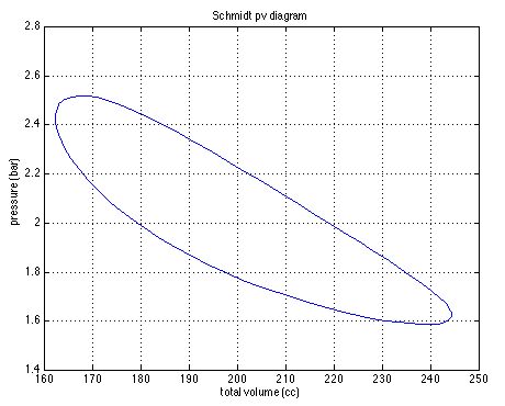
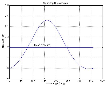
plotpv is invoked to
do Schmidt analysis pV and p-theta diagrams, typically as follows:
|
|
|
function plotpv
% plot pv and p-theta diagrams of Schmidt analysis
% Israel Urieli 1/6/03
global vclc vcle % compression,expansion clearence vols [m^3]
global vswc vswe % compression, expansion swept volumes [m^3]
global alpha % phase angle advance of expansion space [radians]
global vk % cooler void volume [m^3]
global vh % heater void volume [m^3]
global vr % regen void volume [m^3]
global mgas % total mass of gas in engine [kg]
global rgas % gas constant [J/kg.K]
global pmean % mean (charge) pressure [Pa]
global tk tr th % cooler, regenerator, heater temperatures [K]
theta = 0:5:360;
vc = vclc + 0.5*vswc*(1 + cos(theta*pi/180));
ve = vcle + 0.5*vswe*(1 + cos(theta*pi/180 + alpha));
p = mgas*rgas./(vc/tk + vk/tk + vr/tr + vh/th + ve/th)*1e-5; % [bar]
vtot = (vc + vk + vr + vh + ve)*1e6; % [cc]
figure
plot(vtot,p)
grid on
xlabel('total volume (cc)')
ylabel('pressure (bar)')
title('Schmidt pv diagram')
figure
plot(theta,p)
grid on
hold on
x = [0,360];
y = [pmean*1e-5, pmean*1e-5];
plot(x,y)
xlabel('crank angle (deg)')
ylabel('pressure (bar)')
title('Schmidt p-theta diagram')
|
______________________________________________________________________________________
![]()
Stirling Cycle Machine Analysis by
Israel
Urieli is licensed under a Creative
Commons Attribution-Noncommercial-Share Alike 3.0 United States
License