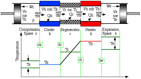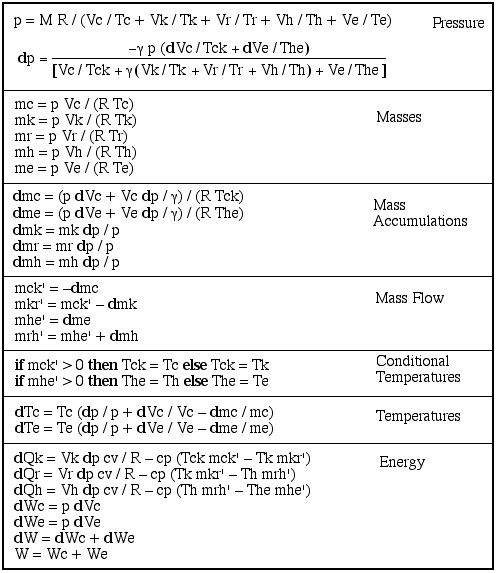


We now consider the solution of the equation set above. Because of the non-linear nature of the equations (in particular with regards to the Conditional Temperatures) we have to resort to a numerical solution of specific configurations and operating conditions.
The specific engine configuration and geometry defines Vc, Ve, dVc, and dVe as analytic functions of the crankangle θ, and the heat exchanger geometry defines the void volumes Vk, Vr, Vh. The choice of working gas (typically air, helium or hydrogen) specifies R, cp, cv, and γ. The operating conditions specify Tk and Th, and thus the mean effective temperature Tr = (Th - Tk) / ln(Th / Tk). Specifying the total mass of working gas M is a problem, since this is not normally a known parameter. The approach we use is to specify the mean operating pressure pmean and then use the Schmidt Analysis to evaluate M. Even though the Ideal Adiabatic model is independent of operating frequency, we nevertheless specify it in order to evaluate power and other time related effects (such as thermal conduction loss in the regenerator housing.)
We notice that apart from the constant parameters specified above, there are 22 variables and 16 derivatives in the equation set, to be solved over a complete cycle (θ = [0, 2π]):
Tc, Te, Qk, Qr, Qh, Wc, We - seven derivatives to be integrated numerically
W, p, Vc, Ve, mc, mk, mr, mh, me - nine analytical variables and derivatives
Tck, The, mck', mkr', mrh', mhe' - six conditional and mass flow variables (derivatives undefined)
We treat this as a "quasi steady-flow" system, thus over each integration interval the four mass flow variables mck', mkr', mrh', and mhe' remain constant and there are no acceleration effects. Thus we consider the problem as that of solving a set of seven simultaneous ordinary differential equations.
The simplest approach to solving a set of ordinary differential equations is to formulate it as an initial-value problem, in which the initial values of all the variables are known and the equations are integrated from that initial state over a complete cycle. The initial value problem can be stated in simple terms. Let the vector Y collectively represent the seven unknown variables, thus y[Tc] is the compression space temperature, y[We] is the work done by the expansion space, and so on. Given an initial condition Y(θ = 0) = Y0 and the corresponding set of differential equations dY = F(θ, Y), evaluate the unknown functions Y(θ) that satisfy both the differential equations and the initial conditions. A numerical solution to this problem is accomplished by first computing the values of the derivatives at θ0 and proceding in small increments of θ to a new point θ1 = θ0 + Δθ. Thus the solution is composed of a series of short straight-line segments that approximate the true curves Y(θ). Among the vast number of methods available for solving initial-value problems, the classical fourth-order Runge-Kutta method is probably the most frequently used.
In order to develop our specific method of solution of the initial-value problem, we have presented a case study in the MATLAB language involving a large-angle pendulum. We do not use the MATLAB built-in functions for solving ordinary differential equations, since our method requires overloading features not available in these built-in functions.
Unfortunately the Ideal Adiabatic model is not an initial-value problem, but is instead a boundary-value problem. We do not know the initial values of the working space gas temperatures Tc and Te, which result from the adiabatic compression and expansion processes as well as enthalpy flow processes. The only guidance that we have to their correct choice is that their values at the end of the steady-state cycle should be equal to their respective values at the beginning of the cycle.
However, because of its cyclic nature, the system can be formed as an initial value problem by assigning arbitrary initial conditions, and integrating the equations through several complete cycles until a cyclic steady state has been attained. This is equivalent to the transient "warm-up" operation of an actual machine. Experience has shown that the most sensitive measure of convergence to cyclic steady state is the residual regenerator heat Qr at the end of the cycle, which should be zero.
The compression and expansion space temperatures are thus initially specified at Tk and Th respectively. The system of equations can then be solved through as many cycles as necessary in order to attain cyclic steady state. For most configurations, between five and ten cycles will be sufficient for convergence.
______________________________________________________________________________________
![]()
Stirling Cycle Machine Analysis by Israel
Urieli is licensed under a Creative
Commons Attribution-Noncommercial-Share Alike 3.0 United States
License