Chapter 8 The Logic of Hypothesis Testing

All of us hypothesize all the time. We look at the world around us, something that happened yesterday or might happen tomorrow, and try to concoct a story in our head about the chance of yesterday’s/tomorrow’s event happening. We may even weave together a silent, internalized narrative about how the event came about. These stories in our head are conjectures, our best guesses, maybe even biased thoughts, but they have not been tested with data. For example, you may be a city employee in the Streets and Sanitation department who feels the city has gotten dirtier over the past five years. You may be an admissions counselor who thinks the academic preparation of the pool of high school graduates applying to your university has gotten better over the years. Maybe you work as a program evaluation specialist in the Ohio Department of Education and need to find out if a dropout recovery program has made any difference in reducing high-school dropout rates. These suspicions, the motivating questions, are hypotheses that have not yet been tested with data. If you were keen to test your hypothesis, you would have to follow an established protocol that starts with a clear articulation of the hypotheses to be tested. Formally, we define hypothesis testing as an inferential procedure that uses sample data to evaluate the credibility of a hypothesis about a population parameter. The process involves (i) stating a hypothesis, (ii) drawing a sample to test the hypothesis, and (iii) carrying out the test to see if the hypothesis should be rejected (or not). Before we proceed, however, memorize the following statement: A hypothesis is an assumption that can neither be proven nor disproven without a reasonable shadow of doubt, a point that will become all too clear by the time we end this chapter.¹⁰

8.1 Articulating the Hypotheses to be tested

Hypotheses are denoted by $H$, for example,

$H$: Not more than 5% of GM trucks breakdown in under 10,000 miles
$H$: Heights of North American adult males is distributed with $\mu = 72$ inches
$H$: Mean year-round temperature in Athens (OH) is $> 62$
$H$: 10% of Ohio teachers have the highest rating (Accomplished)
$H$: Mean county unemployment rate in an Appalachian county is 12.1%
$H$: The Dropout Recovery program has reduced average dropout rates to be no higher than 30%

Hypotheses come in pairs, one the null hypothesis and the other the alternative hypothesis. The null hypothesis, often denoted as $H_{0}$, is the assumption believed to be true while the alternative hypothesis, often denoted as $H_{a}$ or $H_{1}$ is the statement believed to be true if $H_{0}$ is rejected by the statistical test. Some expressions follow, all in the context of average heights of adult males in North America

$H_{0}$: $\mu > 72$ inches; $H_{1}$: $\mu \leq 72$
$H_{0}$: $\mu < 72$ inches; $H_{1}$: $\mu \geq 72$
$H_{0}$: $\mu \leq 72$ inches; $H_{1}$: $\mu > 72$
$H_{0}$: $\mu \geq 72$ inches; $H_{1}$: $\mu < 72$
$H_{0}$: $\mu = 72$ inches; $H_{1}$: $\mu \neq 72$

$H_{0}$ and $H_{1}$ are mutually exclusive and exhaustive, mutually exclusive in the sense that either $H_{0}$ or $H_{1}$ can be true at a given point in time (both cannot be true at the same point in time), and exhaustive in that $H_{0} + H_{1}$ exhaust the sample space (there is no third or fourth possibility unknown to us).

When we setup our null and alternative hypotheses we must pay careful attention to how we word each hypothesis. In particular, we usually want the alternative hypothesis to be the one we hope is supported by the data and the statistical test while the null hypothesis is the one to be rejected. Why? Because rejecting the null implies the alternative must be true. As a rule, then, always setup the alternative hypothesis first and then setup the null hypothesis. For example, say I suspect that dropout rates have dropped below 30% and I hope to find this suspicion supported by the test. I would then setup the hypotheses as follows:

\[\begin{array}{l} H_0: \text{ mean dropout rate } \geq 30\% \\ H_1: \text{ mean dropout rate } < 30\% \end{array}\]

If I don’t know whether dropout rates have decreased or increased, I just suspect they are not what they were last year (which may have been, say, 50%), then I would set these up as follows:

\[\begin{array}{l} H_0: \text{ mean dropout rate } = 50\% \\ H_1: \text{ mean dropout rate } \neq 50\% \end{array}\]

Notice the difference between the two pairs of statements. On the first pass I had a specific suspicion, that rates had fallen below 30% and so I setup the hypotheses with this specificity in mind. On the second go around I had less information to work with, just a feeling that they weren’t 50% and hence I setup less specific hypotheses. This leads us to a very important point you should always bear in mind: Hypotheses testing is only as good as the underlying substantive knowledge used to develop the hypotheses. If you know nothing about the subject you are researching, your hypothesis development will be blind to reality and the resulting $H_0$ and $H_1$ almost guaranteed to be incorrectly setup. There is thus no substitute to reading as widely as possible before you embark on sampling and hypothesis testing.

8.2 Type I and Type II Errors

Hypothesis testing is fraught with the danger of drawing the wrong conclusion, and this is true in all research settings. This means that whenever you reject a null hypothesis, there is always some non-zero probability, however small it may be, that in fact you should not have rejected the null hypothesis. Similarly, every time you fail to reject the null hypothesis there is always some non-zero probability that in fact you should have rejected the null hypothesis. Why does this happen? It happens because we do not see the population and are forced to work with the sample we drew, and samples can mislead us by sheer chance. Let us formalize this tricky situation.

Assume there are two states of the world, one where the null hypothesis is true (but we don’t know this) and the other where the null hypothesis is false (but we don’t know this).

TABLE 8.1: Type I and Type II Errors
Decision based on Sample	Null is true	Null is false
Reject the Null	Type I error	No error
Do not reject the Null	No error	Type II error

The correct decisions are shown in the green cells while the incorrect decisions are shown in the red cells. The two errors that could happen are labeled Type I and Type II errors, respectively. A Type I error is a false positive and occurs if you reject the null hypothesis when you shouldn’t have, and a Type II error is a false negative and occurs if you fail to reject the null hypothesis when you should have. When we carry out a hypothesis test we usually default to minimizing the probability of a Type I error but in some cases the probability of a Type II error may be the one we wish to minimize. Both cannot be minimized at the same time. Why these errors are omnipresent in every hypothesis test and why both cannot be minimized at the same time will become clear once we do a few hypothesis tests.

The probability of a Type I error given that the null hypothesis is true is labeled $\alpha$ and the probability of a Type II error given that the null hypothesis is false is labeled $\beta$. The probability of correctly rejecting a false null hypothesis equals $1- \beta$ and is called the power of a test. Estimating the power of a test is a fairly complicated task and taken up in some detail in a later Chapter.

We also refer to $\alpha$ as the level of significance of a test, and conventionally two values are used for $\alpha$, $\alpha = 0.05$ and $\alpha = 0.01$. With $\alpha = 0.05$ we are saying we are comfortable with a false positive, with rejecting the null hypothesis when we shouldn’t have, in at most five out of every 100 tests of the same hypotheses with similarly sized random samples. With $\alpha = 0.01$ we are saying we are comfortable with a false positive, with rejecting the null hypothesis when we shouldn’t have, in at most one out of every 100 tests of the same hypotheses with similarly sized random samples. If you want a lower false positive rate then go with $\alpha = 0.01$. There is a trade-off, however: If you choose a lower false positive rate $(\alpha = 0.01)$ then it will generally be harder to reject the null hypothesis than it would have been with a higher false positive rate $(\alpha = 0.05)$.

8.3 The Process of Hypothesis Testing: An Example

Assume we want to know whether the roundabout on SR682 in Athens, Ohio, has had an impact on traffic accidents in Athens. We have historical data on the number of accidents in years past. Say the average per day used to be 6 (i.e., $\mu = 6$). To see if the roundabout has had an impact, we could gather accident data for a random sample of 100 days $(n=100)$ from the period after the roundabout was built. Before we do that though, we will need to specify our hypotheses. What do we think might be the impact? Let us say the City Engineer argues that the roundabout should have decreased accidents. If he is correct then the sample mean ($\bar{x}$) should be less than the population mean ($\mu$) i.e., $\bar{x} < \mu$. If he is wrong then the sample mean ($\bar{x}$) should be at least as much as the population mean ($\mu$) i.e., $\bar{x} \geq \mu$.

We know from the theory of sampling distributions that the distribution of sample means, for all samples of size $n$, will be normally distributed. Most sample means would be in the middle of the distribution but, of course, we know that by sheer chance we could end up with a sample mean from the tails (the upper and lower extremes of the distribution). This will happen with a very small probability but it could happen, so bear this possibility in mind. The sampling distribution is shown below:

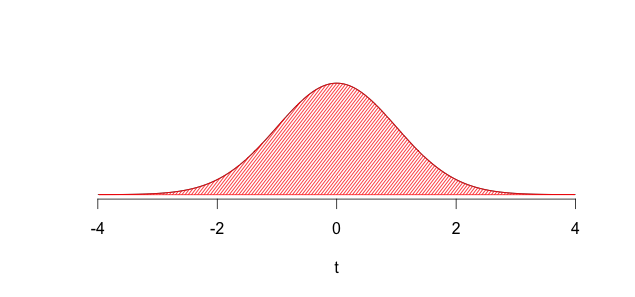
FIGURE 8.1: Sampling Distribution of Mean Traffic Accidents

If we believe the City Engineer, we would setup the hypotheses as $H_0$: The roundabout does not reduce accidents, i.e., $\mu \geq \mu_0$, and $H_1$: The roundabout does reduce accidents, i.e., $\mu < \mu_0$.

We then calculate the sample mean $(\bar{x})$ and the sample standard deviation $(s)$, then the standard error of the sample mean: $s_{\bar{x}} = \dfrac{s}{\sqrt{n}}$, and finally the $t_{calculated} = \dfrac{\bar{x} - \mu}{s_{\bar{x}}}$. The next step would involve using $df=n-1$ and finding the area to the left of $t_{calculated})$. If this area were very small then we could conclude that the roundabout must have worked to reduce accidents. How should we define ``very small’’? By setting $\alpha$ either to 0.05 or to 0.01. Once we set $\alpha$ we would Reject $H_0$ if $P(t_{calculated}) \leq \alpha$ because this would imply that the probability of getting a $t$ value such as the one we calculated so far from the middle of the distribution, by sheer chance, is very small. Thus our findings must be reliable, the data must be providing sufficient evidence to conclude that the roundabout has reduced accidents. If, however, $P(t_{calculated}) > \alpha$ then we would Fail to reject $H_0$; the data would be providing us with insufficient evidence to conclude that the roundabout has reduced accidents.

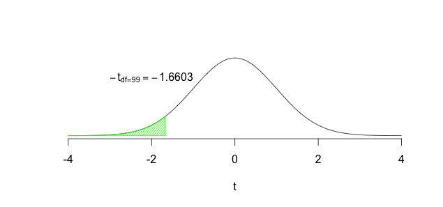
FIGURE 8.2: Rejecting the Null

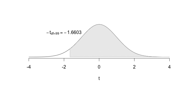
FIGURE 8.3: Failing to Reject the Null

In the plots above, the green region in the figure shows where we need our calculated $t$ to fall before we can reject the null hypothesis, and the grey region shows the area where we need our calculated $t$ to fall if we are not rejecting the null hypothesis. The green region is often referred to as the critical region or the rejection region.

What if the City Engineer had no clue whether accidents might have decreased or increased? Well, in that case we would we would setup the hypotheses as $H_0$: The roundabout has no impact on accidents, i.e., $\mu = \mu_0$, and $H_1$: The roundabout has an impact on accidents, i.e., $\mu \neq \mu_0$. Next steps would be to calculate the sample mean $(\bar{x})$ and the sample standard deviation $(s)$, followed by the standard error of the sample mean: $s_{\bar{x}} = \dfrac{s}{\sqrt{n}}$, then $t_{calculated} = \dfrac{\bar{x} - \mu}{s_{\bar{x}}}$. Using $df=n-1$, we would then find the area to the left/right of $\pm t_{calculated})$. If this area were very small we would conclude that the roundabout must have worked to reduce accidents. Once again, how should we define “very small?” By setting $\alpha$ either to 0.05 or to 0.01. We could then Reject $H_0$ if $P(\pm t_{calculated}) \leq \alpha$; the data would be providing us with sufficient evidence to conclude that the roundabout had an impact on accidents. If $P(\pm t_{calculated}) > \alpha$ then we would Fail to reject $H_0$; the data would be providing us with insufficient evidence to conclude that the roundabout had an impact on accidents. Watch the plots below to see the critical region in this particular scenario.

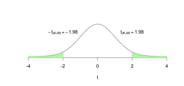
FIGURE 8.4: Rejecting the Null

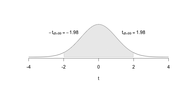
FIGURE 8.5: Failing to Reject the Null

Note the difference between the first time we tested the City Engineer’s suspicions and the second time we did so.

In the first instance he/she had a very specific hypothesis, that accidents would have decreased. This led us to specify $H_1: \mu < \mu_{0}$. Given the inequality $<$ we focused only on the left side of the distribution to decide whether to reject the null hypothesis or not.
In the second instance he/she had a vague hypothesis, that accidents will occur at a different rate post-construction of the roundabout. This led us to specify $H_1: \mu \neq \mu_{0}$. Given the possibility that accidents could have increased/decreased, we now focused on both sides of the distribution (left and right) to decide whether to reject the null hypothesis or not.

Hypothesis tests of the first kind are what we call one-tailed tests and those of the second kind are what we call two-tailed tests. Once we do a few hypothesis tests I will explain how two-tailed tests require more evidence from your data in order to reject the null hypothesis; one-tailed tests make it relatively easier to reject the null hypothesis. For now, here is recipe for specifying hypotheses …

State the hypotheses
- If we want to test whether something has “changed” then $H_0$ must specify that nothing has changed $\ldots H_0:\mu = \mu_{0}; H_1: \mu \neq \mu_{0} \ldots$ two-tailed
- If we want to test whether something is “different” then $H_0$ must specify that nothing is different $\ldots H_0:\mu = \mu_{0}; H_1: \mu \neq \mu_{0}\ldots$ two-tailed
- If we want to test whether something had an “impact” then $H_0$ must specify that it had no impact $\ldots H_0:\mu = \mu_{0}; H_1: \mu \neq \mu_{0}\ldots$ {two-tailed}
- If we want to test whether something has “increased” then $H_0$ must specify that it has not increased $\ldots H_0:\mu \leq \mu_{0}; H_1: \mu > \mu_{0}\ldots$ {one-tailed}
- If we want to test whether something has “decreased” then $H_0$ must specify that it has not decreased $\ldots H_0:\mu \geq \mu_{0}; H_1: \mu < \mu_{0}\ldots$ {one-tailed}
Collect the sample and set $\alpha=0.05$ or $\alpha=0.01$
Calculate $s_{\bar{x}} = \dfrac{s}{\sqrt{n}}$, $\bar{x}$, $df=n-1$
Calculate the $t$
Reject $H_0$ if calculated $t$ falls in the critical region; do not reject $H_0$ otherwise

8.3.1 Example 1

Last year, Normal (IL) the city’s motor pool maintained the city’s fleet of vehicles at an average cost of $\$346$ per car. This year Jack’s Crash Shop is doing the maintenance. The city engineer notices that in a random sample of 36 cars repaired by Jack, the mean repair cost is $\$330$ with a standard deviation of $\$120$. Is going with Jack saving the city money?

Here are the hypotheses: $H_0: \mu \geq 346$ and $H_1: \mu < 346$

Let us choose $\alpha = 0.05$ and calculate the degrees of freedom: $df=n-1=36-1=35$. We need the standard error so let us calculate that: $s_{\bar{x}} = \dfrac{s}{\sqrt{n}} = \dfrac{120}{\sqrt{36}} = 20$. The calculated $t$ will be $t = \dfrac{\bar{x} - \mu_{0}}{s_{\bar{x}}} = \dfrac{330-346}{20} = \dfrac{-16}{20} = -0.80$

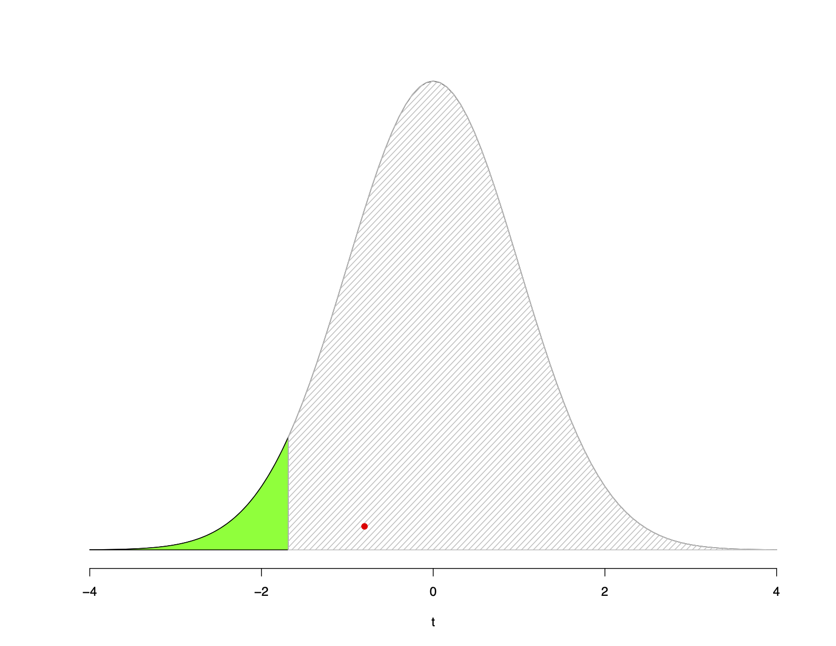
FIGURE 8.6: Example 1

The green area shows the critical region, while the gray area shows the rest of the distribution. The red dot shows where our calculated $t = -0.80$ falls. Since it does not fall in the critical region we fail to reject $H_0$. The data provide insufficient evidence to conclude that going with Jack’s shop is saving the city money.

How did we find the critical region? We found it by looking up what we call the critical t value for given degrees of freedom. Here we have $df = 35$. If I use an online table for finding $t$ values and areas under the distribution, like the one here, I see that the critical region starts at $t=-1.69$ and extends left to the end of the distribution’s left-tail. This is the green area in the plot.

So another way of deciding whether to reject the null or not is to compare the calculated $t$ to the critical $t$ using the following guidelines:

$H_1: \mu < \mu_{0}$, reject $H_0$ if $-t_{calculated} \leq -t_{critical}$
$H_1: \mu > \mu_{0}$, reject $H_0$ if $t_{calculated} \geq t_{critical}$
$H_1: \mu \neq \mu_{0}$, reject $H_0$ if $\lvert{t_{calculated}}\rvert \geq \lvert{t_{critical}}\rvert$ Using this rule, my calculated $t = -0.80$ is not less than or equal to the critical $t = -1.69$ and so I cannot reject the null hypothesis.

I could have also just looked up my calculated $t$ and then found $P(t \leq -0.80)$. If this area were smaller than $\alpha$, I could reject the null hypothesis. If this area were greater than $\alpha$ I would fail to reject the null hypothesis. Using the online table if I enter values for the calculated $t$ and the degrees of freedom I see the area to be $0.2146$. This is quite a bit larger than $\alpha = 0.05$ so I fail to reject the null hypothesis. This is the more common way of making decisions about hypothesis tests so let us memorize this rule:

$P(t \leq t_{calculated}) \leq \alpha$: Reject the null hypothesis
$P(t \leq t_{calculated}) > \alpha$: Do not reject the null hypothesis

8.3.2 Example 2

Kramer’s (TX) Police Chief learns that her staff clear 46.2% of all burglaries in the city. She wants to benchmark their performance and to do this she samples 10 other demographically similar cities in Texas. She finds their clearance rates to be as follows:


44.2	32.1
40.3	32.9
36.4	29.0
49.4	46.4
51.7	41.0

Is Kramer’s clearance rate significantly different from those of other similar Texas cities?

$H_0: \mu = 46.2$ and $H_1: \mu \neq 46.2$.

Set $\alpha = 0.05$ and note $df=n-1=10-1=9$, $\bar{x}=40.34$, and $s_{\bar{x}} = 2.4279$

$t = \dfrac{ \bar{x} - \mu_{0} }{ s_{\bar{x}} } = \dfrac{40.34-46.2}{2.4279} = -2.414$

Critical $t = \lvert{2.262}\rvert$. Our calculated $t = -2.414$ clearly surpasses critical $t$ and so we can reject the null hypothesis; Kramer’s clearance rate seems to be different from that of demographically similar cities.

If I looked up $P(t \leq t_{calculated})$ I would find this to be $0.039$. Since this is less than $\alpha = 0.05$ I can easily reject the null hypothesis. The graphical depiction of the decision is shown below:

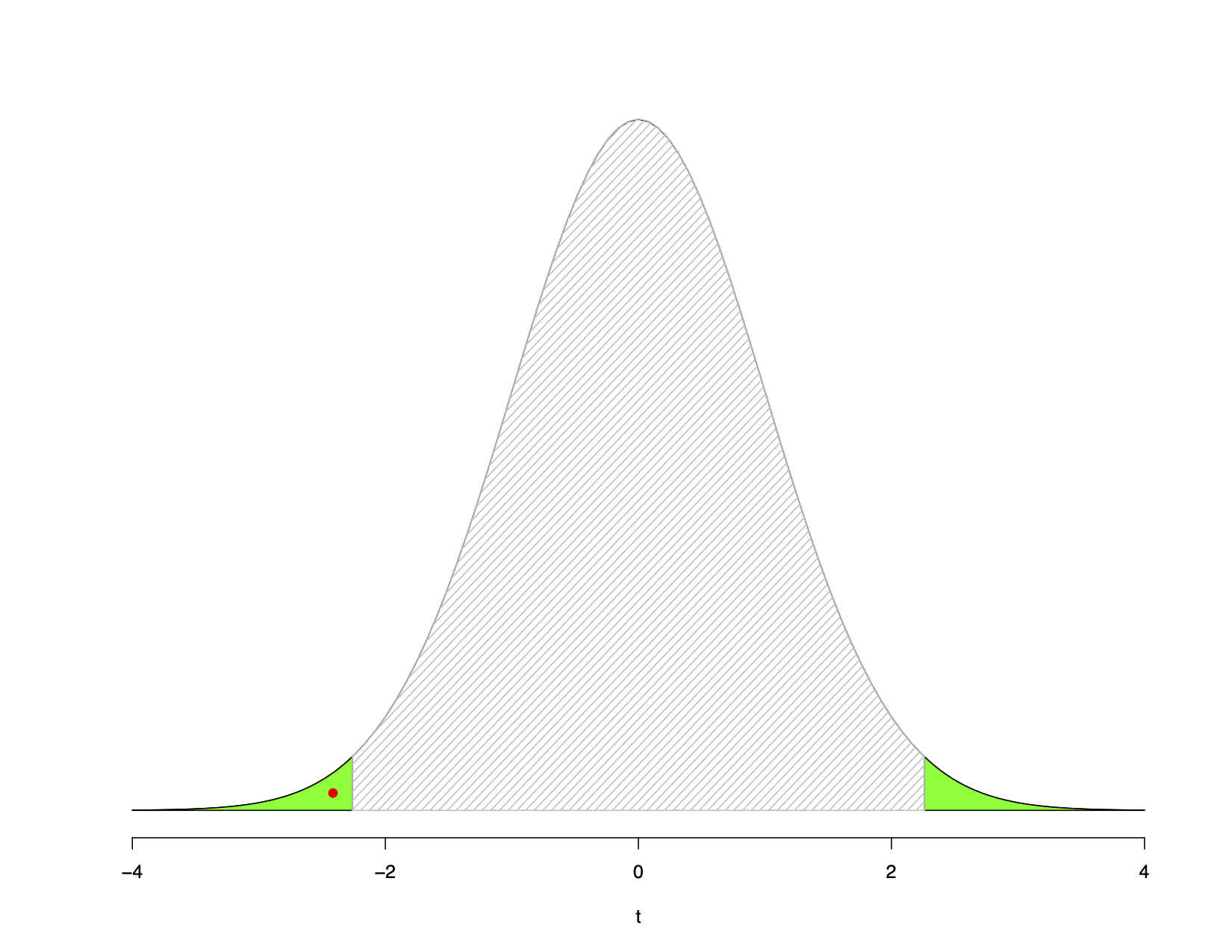
FIGURE 8.7: Example 2

8.4 Confidence Intervals for Hypothesis Tests

Confidence intervals can and should be used for hypothesis tests as well because they are more informative than simply providing the sample mean and our decision about rejecting/not rejecting the null hypothesis. They are used as follows:

Calculate the appropriate confidence interval for the $\alpha$ used for the hypothesis test. This interval will be calculated for the sample mean (or proportion).
See if the confidence interval traps the null value used in the hypotheses. If it does, then the null should not be rejected. If it does not, then the null should be rejected.

Let us take the Kramer (TX) example for demonstration purposes. Our sample mean was 40.34 and the population mean was 46.2, the standard error was 2.4279, the critical $t$ was 2.262, and $\alpha$ was 0.05. Consequently, the, 95% interval would be $40.34 \pm 2.262(2.4279) = 40.34 \pm 5.49191 = 34.84809 \text{ and } 45.83191$. Note that the value of 46.2 does not fall in this interval and hence we can reject the null hypothesis.

If you calculate the appropriate interval for Jack’s Crash Shop in Example 1 you will see the two-tail critical value being $\pm 2.03224451$ and the resulting interval calculated as 289.3551 and 370.6449. In Example 1 we failed to reject the null hypothesis. Since our confidence interval includes the population value of 346 we fail to reject the null here as well.

As a rule, then, if you are able to reject the null hypothesis your confidence interval will not subsume the population value used in the null hypothesis. Likewise, if you are unable to reject the null hypothesis your confidence interval will not subsume the population value used in the null hypothesis.

8.5 The One-Sample t-test

The preceding hypothesis tests are what we call a one-sample t-test where we have a population mean, a single sample to work with, and are looking to test whether the sample mean differs from the population mean. These tests are built upon some assumptions and if these assumptions are violated the test-based conclusions become wholly unreliable.

8.5.1 Assumptions

The assumptions that apply to the one-sample t-test are:

The variable being tested is an interval-level or ratio-level measure
The data represent a random sample
There are no significant outliers
The variable(s) being tested are approximately normally distributed

The random sample assumption we generally hold to be true because if we knew we had messed up and ended up with a non-random sample, I hope we would be smart enough to avoid doing any kind of a statistical test altogether. Similarly, one would (hopefully) know that our measures were neither interval nor ratio-level and hence we should not do a t-test. The assumptions that need to be tested are thus those of normality and significant outliers. We will do these shortly.

8.6 The Two-group (or Two-sample) t-test

The more interesting tests involve two groups such as, for example, comparing reading proficiency levels across male and female students, studying the wage gap between men and women, seeing if the outcome differs between those given some medicine versus those given a placebo, and so on. The logic underlying the hypothesis test is simple: If both groups come from a common population, their means should be identical Of course, the means could differ a little by chance but a large difference in the means would happen with a small probability. If this probability is less than or equal to the test $\alpha$, we reject the null hypothesis.If this probability is greater than the test $\alpha$ we do not reject the null hypothesis. Let us see this logic by way of a visual representation.

In the plot below you see the bell-shaped distribution that characterizes the population and two dots, the red marking the mean reading score for female students and the blue marking the mean reading score for male students. Both are identical; $\mu_{female} = \mu_{male}$, and this would be true if there was no difference between the two groups.

FIGURE 8.8: A Normal Distribution

You could, of course, end up seeing the means some distance apart purely by chance even though in the population there is no difference between the groups. This is shown for four stylized situations although the possibilities of how far apart the means might be are countless.

FIGURE 8.9: Common Parent Population

Since chance can yield the two means some distance apart, the hypothesis test is designed to help us determine whether chance is driving the drift we see or is it really the case that the groups come from separate populations. If they do come from different populations, we would expect to see the following:

FIGURE 8.10: Separate Parent Populations

Note that here the sample means are in the middle of their respective distributions, exactly what you would expect to see in most of your sample. The question thus becomes whether any differences in sample means that we see should be attributed to chance or to the rejection of the belief that both groups share a common parent population. The hypotheses are setup as shown below:

Two-Tailed Hypotheses: $H_0$: $\mu_{1} = \mu_{2}$; $H_A$: $\mu_{1} \neq \mu_{2}$ and these can be rewritten as $H_0$: $\mu_{1} - \mu_{2} = 0$; $H_A$: $\mu_{1} - \mu_{2} \neq 0$
One-Tailed Hypotheses: $H_0$: $\mu_{1} \leq \mu_{2}$; $H_A$: $\mu_{1} > \mu_{2}$, rewritten as $H_0$: $\mu_{1} - \mu_{2} \leq 0$; $H_A$: $\mu_{1} - \mu_{2} > 0$
One-Tailed Hypotheses: $H_0$: $\mu_{1} \geq \mu_{2}$; $H_A$: $\mu_{1} < \mu_{2}$, rewritten as $H_0$: $\mu_{1} - \mu_{2} \geq 0$; $H_A$: $\mu_{1} - \mu_{2} < 0$

The test static is $t = \dfrac{\left(\bar{x}_{1} - \bar{x}_{2} \right) - \left(\mu_{1} - \mu_{2} \right)}{SE_{\bar{x}_{1} - \bar{x}_{2}}}$, with $x_1$ and $x_2$ representing the sample means of group 1 and group 2, respectively.

Given that we have two groups we calculate the standard errors and the degrees of freedom in a more nuanced manner. In particular, we have to decide whether, assuming the null hypothesis to be true (i.e., the groups do indeed come from two different parent populations), these populations have (i) equal variance, or (ii) unequal variances.

Assuming Equal Variances

With equal population variances, we calculate the standard error as:

\[s_{\bar{x}_1 - \bar{x}_2} = \sqrt{\dfrac{n_1 + n_2}{n_1n_2}}\sqrt{\dfrac{(n_1 -1)s^{2}_{x_{1}} + (n_2 -1)s^{2}_{x_2}}{\left(n_1 + n_2\right) -2}}\]

and the degrees of freedom are $df = n_1 + n_2 - 2$. Note that $s^{2}_{x_1}$ and $s^{2}_{x_2}$ are the variances of group 1 and group 2, respectively, while $n-1$ and $n_2$ are the sample sizes of groups 1 and 2, respectively.

Assuming Unequal Variances

With unequal populations variances things get somewhat tricky because now we calculate the standard error as

\[s_{\bar{x}_1 - \bar{x}_2} = \sqrt{\dfrac{s^{2}_{x_1}}{n_1} + \dfrac{s^{2}_{x_2}}{n_2}}\]

and the approximate degrees of freedom as

\[\dfrac{\left(\dfrac{s^{2}_{x_1}}{n_1} + \dfrac{s^{2}_{x_2}}{n_2} \right)^2}{\dfrac{1}{(n_1 -1)}\left(\dfrac{s^{2}_{x_1}}{n_1}\right)^2 + \dfrac{1}{(n_2 -1)}\left(\dfrac{s^{2}_{x_2}}{n_2}\right)^2}\]

These degrees of freedom are derived from the Welch-Satterthwaite equation, named for its authors, and hence the two-group t-test with unequal variances assumed is also called Welch's t-test.

Once again, regardless of equal or unequal variances assumed, our decision criteria do not change: Reject the null hypothesis if the p-value of the calculated $t$ is $\leq \alpha$; do not reject otherwise. Let us see a few examples, although I will not manually calculate the standard errors or degrees of freedom since these days statistical software would be used de jure.

Assumptions

The two-group t-test is driven by some assumptions.

Random samples … usually assumed to be true otherwise there would be no point to doing any statistical test
Variables are drawn from normally distributed Populations … this can be formally tested and we will see how to carry out these tests shortly. However, I wouldn’t worry too much if normality is violated. Bear this in mind.
Variables have equal variances in the Population … this can be formally tested and we will see how to carry out these tests shortly

Although we will be testing two of the assumptions, you may want to bear the following rules of thumb in mind since testing assumptions is not always a cut-and-dried affair.

Draw larger samples if you suspect the Population(s) may be skewed
Go with equal variances if both the following are met:
1. Assumption theoretically justified, standard deviations fairly close
2. $n_1 \geq 30$ and $n_2 \geq 30$
Go with unequal variances if both the following are met:
1. One standard deviation is at least twice the other standard deviation
2. $n_1 < 30$ or $n_2 < 30$

Note also that the t-test is robust in large samples and survives some degree of skewness so long as the skew is of similar degree and direction in each group. How large is “large?” Excellent question but one without a formulaic answer since disciplines define large differently and the sample sample size that someone might see as “small” would appear “large” to others.

8.6.1 Example 1

The Athens County Public Library is trying to keep its bookmobile alive since it reaches readers who otherwise may not use the library. One of the library employees decides to conduct an experiment, running advertisements in 50 areas served by the bookmobile and not running advertisements in 50 other areas also served by the bookmobile. After one month, circulation counts of books are calculated and mean circulation counts are found to be 526 books for the advertisement group with a standard deviation of 125 books and 475 books for the non-advertisement group with a standard deviation of 115 books. Is there a statistically significant difference in mean book circulation between the two groups?

Since we are being asked to test for a “difference” it is a two-tailed test, with hypotheses given by:

\[\begin{array}{l} H_0: \text{ There is no difference in average circulation counts } (\mu_1 = \mu_2) \\ H_1: \text{ There is a difference in average circulation counts } (\mu_1 \neq \mu_2) \end{array}\]

Since both groups have sample sizes that exceed 30 we can proceed with the assumption of equal variances and calculate the standard error and the degrees of freedom. The degrees of freedom as easy: $df = n_1 + n_2 - 2 = 50 + 50 - 2 = 98$. The standard error is $s_{\bar{x}_1 - \bar{x}_2} = \sqrt{\dfrac{n_1 + n_2}{n_1n_2}}\sqrt{\dfrac{(n_1 -1)s^{2}_{x_{1}} + (n_2 -1)s^{2}_{x_2}}{\left(n_1 + n_2\right) -2}}$ and plugging in the values we have

\[s_{\bar{x}_1 - \bar{x}_2} = \sqrt{\dfrac{50 + 50}{2500}} \sqrt{\dfrac{(50 -1)(125^2) + (50 -1)(115^2)}{\left(50 + 50\right) -2}} = (0.2)(120.1041) = 24.02082\]

The test statistic is

\[t = \dfrac{\left( \bar{x}_1 - \bar{x}_2 \right) - \left( \mu_1 - \mu_2 \right) }{s_{\bar{x}_1 - \bar{x}_2}} = \dfrac{(526 - 475) - 0}{24.02082} = \dfrac{51}{24.02082} = 2.123158\]

Since no $\alpha$ is given let us use the conventional starting point of $\alpha = 0.05$. With $df=98$ and $\alpha = 0.05$, two-tailed, the critical $t$ value would be $\pm 1.98446745$. Since our calculated $t = 2.1231$ exceeds the critical $t = 1.9844$, we can easily reject the null hypothesis of no difference. These data suggest there is a difference in average circulation counts between the advertisement and no advertisement groups.

We could have also used the the p-value approach, rejecting the null hypothesis of no difference if the p-value was $\leq \alpha$. The p-value of our calculated $t$ turns out to be 0.0363 and so we can reject the null hypothesis. Note, in passing, that had we used $\alpha = 0.01$ we would have been unable to reject the null hypothesis because $0.0363$ is $> 0.01$.

The 95% confidence interval is given by $(\bar{x}_1 - \bar{x}_2) \pm t_{\alpha/2}(s_{\bar{x}_1 - \bar{x}_2}) = 51 \pm 1.9844(24.02082) = 51 \pm 47.66692 = 3.33308 \text{ and } 98.66692$. We can be about 95% confident that the true difference between the groups lies in this interval. Had we used the 99% interval for a test with $\alpha = 0.01$ the interval would be $51 \pm 2.627(24.02082) = -12.10269 \text{ and } 114.1027$, subsuming the null hypothesis difference of $0$ and leaving us unable to reject the null hypothesis.

8.6.2 Example 2

Say we have a large data-set with a variety of information about several cars, gathered in 1974. One of the questions we have been tasked with testing is whether the miles per gallon yield of manual transmission cars in 1974 was greater than that of automatic transmission cars. Assume they want us to use $\alpha = 0.05$.

We have thirteen manual transmission cars and 19 automatic transmission cars, and the means and standard deviations are 24.3923 and 6.1665 for manual, and 17.1473 and 3.8339 for automatic cars, respectively. The hypotheses are:

\[\begin{array}{l} H_0: \text{Mean mpg of manual cars is } \leq \text{ the mean mpg of automatic cars} (\bar{x}_{man} \leq \bar{x}_{auto}) \\ H_1: \text{Mean mpg of manual cars is } > \text{ the mean mpg of automatic cars} (\bar{x}_{man} > \bar{x}_{auto}) \end{array}\]

The calculated $t$ is 4.1061 and the p-value is 0.0001425, allowing us to reject the null hypothesis. The data suggest that average mpg of manual cars is not not $\leq$ that of automatic cars.

Note a couple of things here: (i) We have a one-tailed hypothesis test, and (ii) we are assuming equal variances since both conditions are not met for assuming unequal variances. In addition, note that the confidence interval is found to be $(3.6415, 10.8483)$, indicating that we can be 95% confident that the average manual mpg is higher than average automatic mpg by anywhere between 3.64 mpg and 10.84 mpg.

8.6.3 Caution

If, for two groups, the confidence intervals around each group mean do not overlap with that of the other group, we can safely infer the two groups are statistically significantly different. Be careful, however, to not automatically infer no statistically significant differences just because the confidence intervals of two groups overlap. Why, you ask? See here and here. This is a common mistake a lot of us slip into.

8.7 Paired t-tests

Assume, for example, that we have measured some outcome for the same set of individuals at two points in time. This situation could be akin to gathering a random sample of $6^{th}$ grade students, recording their mathematics scores on the statewide assessment, and then some years later recording their $8^{th}$ grade mathematics scores on the statewide assessment. We might be curious to know if on average, students’ mathematics performance has improved over time, either organically or because of some special mathematics tutoring program that implemented in the school. Or we may have a situation where the question is whether hospitalization tends to depress patients and so we measure their mental health before hospitalization and then again after hospitalization.

We need not have the same individuals measured twice; paired t-tests also work with two groups with different individuals in each group so long as the groups are similar. What does that mean? Well, think of it as follows. Say I am interested in the hospitalization question. I know that if I administer some mental health assessment (most likely with a battery of survey-type questions) prior to hospitalization, and then I go back with the same battery of questions post-hospitalization, the patients might catch on to the purpose of my study and tailor their responses accordingly. If they don’t respond honestly to my questions, the resulting data will be contaminated. How can I get around this hurdle? A common technique used in situations such as these, where you cannot go back to the same set of individuals, involves finding individuals who are similar to the first group such that both groups have the same average age of the patients, the same proportion of males versus females, similar distributions of income, pre-existing medical conditions, and so on. If we employ such an approach then we have what we call a matched pairs design.

Assumptions

The following assumptions apply to paired t-tests:

Random samples … usually assumed to be true otherwise there would be no point to doing any statistical test
Variables are drawn from normally distributed Populations … this can be formally tested and we will see how to carry out these tests shortly

The Testing Protocol

Let us see how the test is carried out with reference to a small data-set wherein we have six pre-school children’s scores on a vocabulary test before a reading program is introduced into the pre-school $(x_1)$ and then again after the reading program has been in place for a few months $(x_2)$.

TABLE 8.2: Vocabulary Scores pre- and post-intervention
Child ID	Pre-intervention score	Post-intervention score	Difference = Pre - Post
1	6.0	5.4	0.6
2	5.0	5.2	-0.2
3	7.0	6.5	0.5
4	6.2	5.9	0.3
5	6.0	6.0	0.0
6	6.4	5.8	0.6

Note the column $d_i$ has the difference of the scores such that for Child 1, $6.0 - 5.4 = 0.6$, for Child 2, $5.0 - 5.2 = -0.2$, and so on. The mean, variance and standard deviation of $d$ are calculated as follows:

\[\begin{eqnarray*} d_{i} &=& x_{1} - x_{2} \\ \bar{d} &=& \dfrac{\sum{d_i}}{n} \\ s^{2}_{d} &=& \dfrac{\sum(d_i - \bar{d})^2}{n-1} \\ s_d &=& \sqrt{\dfrac{\sum(d_i - \bar{d})^2}{n-1}} \end{eqnarray*}\]

Note also that if the reading program is very effective, then we should see average scores being higher post-intervention, even if some students don’t necessarily improve their individual scores.

Say we have no idea what to expect from the program. In that case, our hypotheses would be:

\[\begin{array}{l} H_0: \mu_d = 0 \\ H_1: \mu_d \neq 0 \end{array}\]

The test statistic is given by $t = \dfrac{\bar{d} - \mu_d}{s_d/\sqrt{n}}; df=n-1$ and the interval estimate calculated as $\bar{d} \pm t_{\alpha/2}\left(\dfrac{s_d}{\sqrt{n}}\right)$.

Once we have specified our hypotheses, selected $\alpha$, and calculated the test statistic, the usual decision rules apply: Reject the null hypothesis if the calculated $p-value \leq \alpha$; do not reject the null hypothesis if the calculated $p-value > \alpha$.

In this particular example, it turns out that $\bar{d}=0.30$; $s_d=0.335$; $t = 2.1958$, ${\circled{\color{blue}{df = 5}}}$, $p-value = 0.07952$ and 95% CI: $0.3 \pm 0.35 = (-0.0512, 0.6512)$.

Given the large $p-value$ we fail to reject $H_0$ and conclude that these data do not suggest a statistically significant impact of the reading program.

8.7.1 Example 1

Over the last decade, has poverty worsened in Ohio’s public school districts? One way to test worsening poverty would be to compare the percent of children living below the poverty line in each school district across two time points. For the sake of convenience I will use two American Community Survey (ACS) data sets that measure Children Characteristics (Table S0901), one the 2011-2015 ACS and the other the 2006-2010 ACS. While a small snippet of the data are shown below for the 35 school districts with data for both years, you can download the full dataset from here.

TABLE 8.3: Percent of Children in Poverty
District	2006-2010	2011-2015
Akron City School District, Ohio	35.3	41.0
Brunswick City School District, Ohio	6.8	7.6
Canton City School District, Ohio	44.1	49.6
Centerville City School District, Ohio	10.5	5.4
Cincinnati City School District, Ohio	39.5	43.0
Cleveland Municipal School District, Ohio	45.8	53.3

\[\begin{array}{l} H_0: \text{ Poverty has not worsened } (d \leq 0) \\ H_1: \text{ Poverty has worsened } (d > 0) \end{array}\]

Subtracting the 2006-2010 poverty rate from the 2011-2015 poverty rate for each district and then calculating the average difference $(d)$ yields $\bar{d} = 4.328571$ and $s_{d} = 3.876746$. With $n=35$ we have a standard error $s_{\bar{d}} = \dfrac{s_d}{\sqrt{n}} = \dfrac{3.876746}{\sqrt{35}} = 0.6552897$. The test statistic is $t = \dfrac{\bar{d}}{s_{\bar{d}}} = \dfrac{4.328571}{0.6552897} = 6.605584$ and has a $p-value = 0.0000001424$, allowing us to easily reject the null hypothesis. These data suggest that school district poverty has indeed worsened over the intervening time period. The 95% confidence interval is $(2.9968 \text{ and } 5.6602)$.

8.7.2 Example 2

A large urban school district in a Midwestern state implemented a reading intervention to boost the district’s scores on the state’s English Language Arts test. The intervention was motivated by poor performance of the district’s $4^{th}$ grade cohort. Three years had passed before that cohort was tested in the $8^{th}$ grade. Did the intervention boost ELA scores, on average?

TABLE 8.4: English Language Arts: Scaled scores, grades Three and Eight
Student ID	Grade	Scaled Score
AA0000001	3	583
AA0000002	3	583
AA0000003	3	583
AA0000004	3	668
AA0000005	3	627
AA0000006	3	617

\[\begin{array}{l} H_0: \text{ Intervention did not boost ELA scores } (d \leq 0) \\ H_1: \text{ Intervention did boost ELA scores } (d > 0) \end{array}\]

We have $\bar{d} = 14.62594$, $s_d = 66.27296$, $df = 12955$ and the standard error is $0.5822609$. The test statistic then is $t = \dfrac{\bar{d}}{s_{\bar{d}}} = \dfrac{14.62594}{0.5822609} = 25.11922$ and has a $p-value$ that is very close to $0$. Hence we can reject the null hypothesis; these data suggest that the reading intervention did indeed boost English Language Arts scores on average.

8.8 Chapter 8 Practice Problems

Problem 1 In the last few years Ohio, like many other states, established a framework for rating teachers and principals/assistant principals. Prior to this policy shift, the existing approach to rating educators yielded very few ineffective teachers, a problem well documented by The Widget Effect. Under the new rating system, the expectation is that the percentage of ineffective teachers will be greater than in the past. Assume that the old system yielded an average of 0.5% of ineffective educators in any school district., (i.e., $\mu = 0.5$). Given this reality, establish the appropriate null and alternative hypotheses.

Assume that your team of program evaluators carries out a statistical test and rejects the null hypothesis. Which error – Type I or Type II – should you be more concerned about?

Explain, in the context of the problem, what committing a Type I error would mean.
Explain, in the context of the problem, what committing a Type II error would mean.

Problem 2

Write the missing hypothesis for each of the hypotheses listed below, both in words and with appropriate mathematical notation:

$H_0$: Average amount of rainfall per year is the same today as what it was in 1977
$H_1$: Adult males’ average heights have increased in recent years
$H_0$: College dropout rates of first generation students are either the same as or lower than those of their non-first generation peers
$H_1$: A human can swim faster in syrup than in water
$H_1$: Average waiting time (in minutes) between eruptions of The Old Faithful geyser exceed 20 minutes
$H_0$: Average number of words typed per minute is not affected by typing tutorials
$H_0$: The number of migrant deaths in Mediterranean waters have not changed since last year

Problem 3

What factor can a research control to reduce the risk of committing a Type I error? What factor can a researcher control to reduce the standard error?

Problem 4

A researcher carried out a one-tailed hypothesis test using $\alpha = 0.01$ and rejected $H_0$. Another researcher repeated the hypothesis test but with $\alpha = 0.05$ and as a two-tailed test, and failed to reject $H_0$. Can both analyses be correct? Explain your answer.

Problem 5

Is crime in America rising or falling? The answer is not as simple as politicians make it out to be because of how the FBI collects crime data from the country’s more than 18,000 police agencies. National estimates can be inconsistent and out of date, as the FBI takes months or years to piece together reports from those agencies that choose to participate in the voluntary program. To try to fill this gap, The Marshall Project collected and analyzed more than 40 years of data on the four major crimes the FBI classifies as violent — homicide, rape, robbery and assault — in 68 police jurisdictions with populations of 250,000 or greater. The research team calculated the rate of crime in each category and for all violent crime, per 100,000 residents in the jurisdiction.

Setup the appropriate hypotheses to test the suggestion that violent crimes per 100,000 (violent_per_100k) exceeded 800 in 2015.
Using $\alpha = 0.05$, carry out the hypothesis test and state your conclusion in words.
Report and interpret the corresponding confidence interval for your estimate of average violent crimes per 100,000 in 2015.

Problem 6

With The Marshall Project data-set, answer the questions that follow .

Setup the hypotheses to test the belief that in 2015, larger cities (defined as cities with population sizes $\geq 500,000$) have more violent crimes per 100,000 than smaller cities (defined as cities with population sizes $< 500,000$). The variable is called total_pop in the data-set.
Carry out the appropriate test and state your conclusion in words. Use $\alpha = 0.01$.
Report and interpret the corresponding confidence interval for your estimated difference in average violent crimes per 100,000 in small versus large cities.

Problem 7

Continuing on with the Marshall Project data-set,

Setup the hypotheses to test the belief that cities’ homicides per 100,000 declined between 1975 and 2015.
Carry out the appropriate test and state your conclusion in words. Use $\alpha = 0.05$.
Report and interpret the corresponding confidence interval for your estimated difference.

Problem 8

The Evidence and Data for Gender Equality (EDGE) project is a joint initiative of the United Nations Statistics Division and UN Women that seeks to improve the integration of gender issues into the regular production of official statistics for better, evidence-based policies. EDGE aims to accelerate existing efforts to generate internationally comparable gender indicators on health, education, employment, entrepreneurship and asset ownership in three many ways, one of which is to develop an online interactive platform to disseminate gender-relevant data on education, employment, and health.

We will focus on the maternal mortality ratio (modeled estimate, per 100,000 live births), available for the 1990 - 2015 period by country and region. You can access this indicator from this file.

Two questions are of interest here:

a belief that in 2015 the average maternal mortality ratio was $< 160$, and
an interest in seeing if on average maternal mortality ratios declined between 1990 and 2015.

Setup the appropriate hypothesis for questions (1) and (2), carry out the test (choose an appropriate value for $\alpha$), state your conclusion in words, and both report and interpret the corresponding confidence interval estimates.

Problem 9

On September $25^{th}$ 2015, countries adopted a set of goals to end poverty, protect the planet, and ensure prosperity for all as part of a new sustainable development agenda. Each goal has specific targets to be achieved over the next 15 years. The World Bank has a wonderful database that provides country-level information on a variety of indicators that feature in The Atlas of Sustainable Development Goals.

Focus on a specific indicator – Access to a mobile phone or internet at home” for males and females aged 15 years old or older, respectively, in 2014. A casual observer suspects that gender discrimination leads to males having differential access a mobile phone or internet at home. Test this suspicion with the data-set available here. State your conclusions, including the interpretation of the confidence intervals for your estimated difference.

Problem 10

The Ohio Department of Education gathers and releases a wealth of data on public schools and community schools; see, for instance, here and here. A snippet of these data are provided for you in this file. Note that you have data for community schools and public school districts; private and parochial schools are excluded.

Thirty-two of our 88 counties are Appalachian, as flagged by the variable Appalachian in the data-set. Focusing on third-grade reading proficiency rates (X3rd.Grade.Reading), test whether the proportion of third-grade students rated proficient or better in reading differs between Appalachian and non-Appalachian districts. Report and interpret your conclusion and the confidence interval for the estimated difference.

Problem 11 The Lalonde data-set with 722 observations on the following 12 variables

age = age in years.
educ = years of schooling.
black = indicator variable for blacks (1 = Black).
hisp = indicator variable for Hispanics (1 = Hispanic).
married = indicator variable for martial status (1 = Married).
nodegr = indicator variable for high school diploma (1 = no high school graduate or equivalent).
re75 = real earnings in 1975.
re78 = real earnings in 1978.
treat = an indicator variable for treatment status (1 = treatment group).

“Key to this data-set is the treatment, which refers to the National Supported Work Demonstration (NSW), a temporary employment program designed to help disadvantaged workers lacking basic job skills move into the labor market by giving them work experience and counseling in a sheltered environment. Unlike other federally sponsored employment and training programs, the NSW program assigned qualified applicants to training positions randomly. Those assigned to the treatment group received all the benefits of the NSW program, while those assigned to the control group were left to fend for themselves.” Lalonde (1986). Note that real earnings in 1975 are before the NSW program began and real earnings in 1978 are the outcome of interest because they were recorded after the NSW treatment had occurred. Using these data answer the following questions:

Did the NSW program have an impact on the real earnings of participants?
Did the NSW program increase the real earnings of participants?

Focusing only on participants in the NSW program,

Did the real earnings in 1978 differ by marital status?
What about between participants with/without a high school degree?

Problem 12

“The Student/Teacher Achievement Ratio (STAR) was a four-year longitudinal class-size study funded by the Tennessee General Assembly and conducted by the State Department of Education. Over 7,000 students in 79 schools were randomly assigned into one of three interventions: small class (13 to 17 students per teacher), regular class (22 to 25 students per teacher), and regular-with-aide class (22 to 25 students with a full-time teacher’s aide). Classroom teachers were also randomly assigned to the classes they would teach. The interventions were initiated as the students entered school in kindergarten and continued through third grade. The Project STAR public access data set contains data on test scores, treatment groups, and student and teacher characteristics for the four years of the experiment, from academic year 1985–1986 to academic year 1988–1989. The test score data analyzed in this chapter are the sum of the scores on the math and reading portion of the Stanford Achievement Test.” Source These data can be downloaded from here. Note the key variables as defined below:

gender = student’s gender 1/male, 2/female
ethnicity = student’s ethnicity 1/caucasian, 2/african-american, 3/asian, 4/hispanic, 5/american-indian, 6/other
stark, star1, star2, star3 = whether the student was in a 2/small classroom, 1/a regular classroom, or 3/a regular classroom with a teaching aide
readk, read1, read2, read3 = reading test scores in kindergarten/grade 1/grade 2/grade 3
mathk, math1, math2, math3 = mathematics test scores in kindergarten/grade 1/grade 2/grade 3
lunchk, lunch1, lunch2, lunch3 = student eligible for free/reduced lunch in kindergarten/grade 1/grade 2/grade 3 with 1/non-free, 2/free
schoolk, school1, school2, school3 = school type student attended in kindergarten/grade 1/grade 2/grade 3 with 1/inner-city, 2/suburban, 3/rural, 4/urban
degreek, degree1, degree2, degree3 = teacher’s highest degree earned in kindergarten/grade 1/grade 2/grade 3 with 1/bachelor, 2/master, 3/specialist, 4/phd
ladderk, ladder1, ladder2, ladder3 = teacher’s career ladder status in kindergarten/grade 1/grade 2/grade 3 with 1/level 1, 2/level 2, 3/level 3, 4/apprentice, 5/probation, 6/pending
experiencek, experience1, experience2, experience3 = teacher’s years of teaching experience in kindergarten/grade 1/grade 2/grade 3
tethnicityk, tethnicity1, tethnicity2, tethnicity3 = teacher’s ethnicity in kindergarten/grade 1/grade 2/grade 3 with 1/caucasian, 2/african-american

Comparing students who were in a small classroom in all four grades to students in a regular classroom in all four grades,

Did reading scores improve between grades k and 3?
What about mathematics scores?

Comparing students who were in a small classroom in all four grades to students in a regular classroom (with our without an aide) in all four grades,

Was there a difference in reading scores in the fourth grade?
What about mathematics scores?

Problem 13

The data for this analysis come from the University of Michigan Panel Study of Income Dynamics (hereafter PSID) for the year 1975 (interview year 1976). Although this year was atypical of most of the 1970’s, only in 1976 did PSID directly interview the wives in the households. During all other years the head of the household’s interview supplied information about the wife’s labor market experiences during the previous year. One suspects that the own reporting is more accurate, and it is for this reason that many recent studies of married women’s labor supply have used these data.

This sample consists of 753 married white women between the ages of 30 and 60 in 1975, with 428 working at some time during the year. This sample size is smaller than most used in the studies reported in Table I. The dependent variable is hours = the wife’s annual hours of work in 1975, and measured as the product of the number of weeks the wife worked for money in 1975 and the average number of hours of work per week during the weeks she worked. The measure of the wage rate is the average hourly earnings, defined by dividing the total labor income of the wife in 1975 by the above measure of her hours of work.

inlf = labor force participation in 1975 = 1
hours = wife’s hours of work in 1975
kidslt6 = number of children less than 6 years old in household
kidsge6 = number of children between ages 6 and 18 in household
age = wife’s age
educ = wife’s educational attainment, in years
wage = wife’s average hourly earnings, in 1975 dollars
repwage = wife’s wage reported at the time of the 1976 interview (not= 1975 estimated wage)
hushrs = husband’s hours worked in 1975
husage = husband’s age
huseduc = husband’s educational attainment, in years
huswage = husband’s wage, in 1975 dollars
faminc = family income, in 1975 dollars
mtr = Federal marginal tax rate facing women
mothereduc = wife’s mother’s educational attainment, in years
fathereduc = wife’s father’s educational attainment, in years
unemprate = unemployment rate in county of residence, in percentage points
city = lives in large city (SMSA) = 1
exper = actual years of wife’s previous labor market experience
nwifeinc = $faminc - (wage \times hours)$ in thousand dollars
lwage = log(wage)
expersq = $exper^2$

Did the wife’s annual hours of work differ according to whether the family lived in a city or not?
Create a new variable $= 1$ if the family had any children under 6 years of age and $= 0$ otherwise. Then test whether the wife’s annual hours of work were greater for families with no children in this age bracket versus at least one child in this age bracket.

Problem 14

The following data-set contains information on 2.725 individuals’ criminal arrest histories. The variables include

narr86 = number of times arrested, 1986
nfarr86 = number of felony arrests, 1986
nparr86 = number property crime arrests, 1986
pcnv = proportion of prior convictions
avgsen = average sentence length, months
tottime = time in prison since 18 (months)
ptime86 = months in prison during 1986
qemp86 = number of quarters employed, 1986
inc86 = legal income, 1986, in hundreds of dollars
durat = recent unemployment duration
black = 1 if Black
hispan = 1 if Hispanic
pcnvsq = pcnv$^2$
pt86sq = ptime86$^2$
inc86sq = inc86$^2$

Was the average sentence length greater for Black versus non-Black individuals?
What about for Hispanic versus non-Hispanic individuals?

It would be remiss of us not to recognize the existence of a very passionate and vigorous Null Hypothesis Significance Testing (NHST) controversy. While the details of the controversy are too advanced for our present purposes, here are some articles you should read: The Truth Wears Off: Is there something wrong with the scientific method? and Do We Really Need the S-word?↩︎