Chapter 11 Linear Regression

In this chapter we close the book with an introduction to regression models – the cornerstone of almost all statistical techniques you see being used in this age of “big data,” “health analytics” and “predictive modeling.” The goal of regression models is to help us understand what variables have a statistically significant impact on some outcome of interest, and how well the regression model we have built can predict outcomes in the future. Imagine, if you will, that you could understand and predict major hurricanes that have hit the United States. If you could accomplish this predictive feat, why then we would know when a hurricane will hit and where, the path it will take, likely damage, the recovery costs, and more. Or perhaps it is a question of delivering better health care and if we can now predict how a patient will respond to total hip or knee surgery, what factors help or hinder speedier recovery, and so on, then patients’ lives will be improved even as health care delivery costs plummet. Indeed, regression models have been used for well over a century now and are employed daily in academia and in the real-world.

11.1 Correlations

The ability to understand how some outcome varies with another event is not rocket science to any of us, even those who have never taken a statistics class. We all understand when two things are correlated because when we see broken windows in a neighborhood we suspect that it is an unsafe neighborhood. Or if we see clouds when we wake up we expect some rainfall before the day is done. What are we doing? Why, recognizing that there seems to be a pattern in that when we see $x$ we often see $y$. Now, just because two things seem to occur at the same time does not mean that one causes another, to claim as such would be disregarding the long-standing adage that correlation is not causation. That is, just because two things are correlated does not mean one causes the other. Look hard enough and you will find ridiculous correlations, a feature of our world that has led to what started as a hilarious website and is now a book: Spurious Correlations. As I write this chapter, the leading spurious correlation Tyler Vigen is displaying is of an almost perfect correlation between U.S. spending on science, technology and space and the number of suicides by hanging, strangulation and suffocation $(r = 0.9978)$.

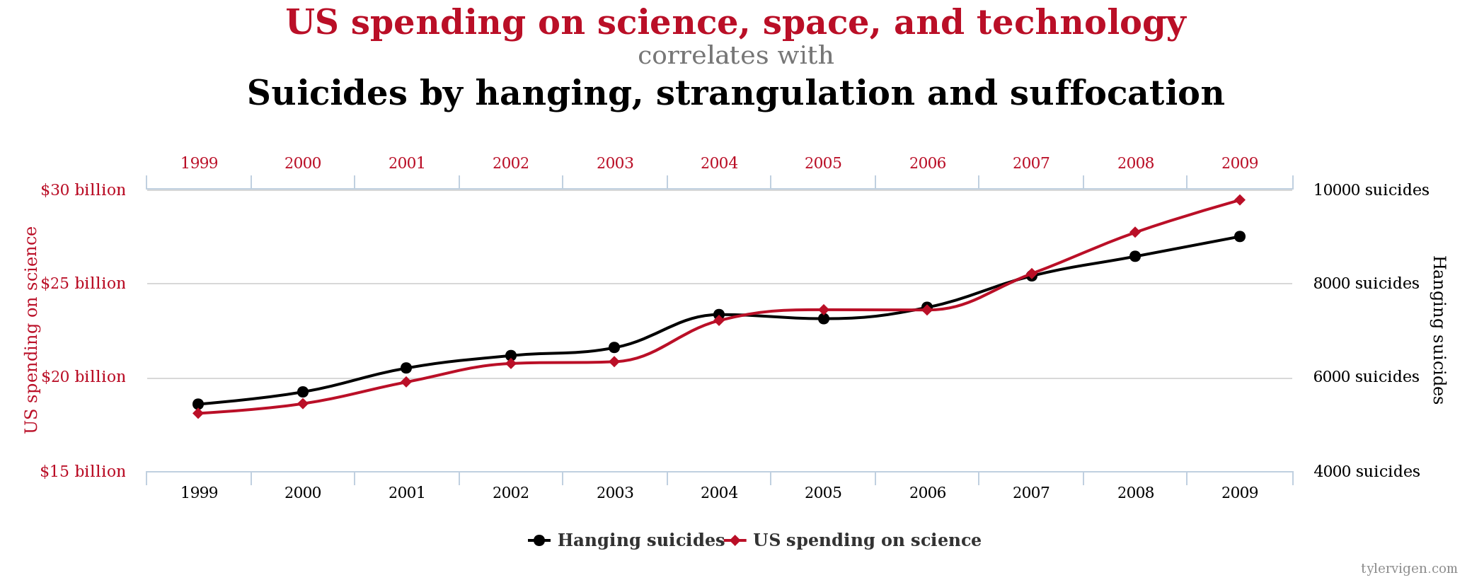
FIGURE 11.1: A Ridiculous Spurious Correlation

So one thing rapidly becomes crystal clear: Correlations do not explain anything, they just reflect a pattern in the data. It is up to us to come up with a plausible explanation for why two things covary. As we allow this point to sink in, we should also recognize that not all correlations are statistically significant. Simply put, we may see two things correlated at $0.5$ but that does not mean the correlation is statistically different from $0$. Let us appreciate these statements in some detail.

11.1.1 Pearson Correlation Coefficient

Given two numeric variables, the degree to which they are correlated is measured via the Pearson Product-Moment Correlation Coefficient, denoted by the symbol $r$. Mathematically, the Pearson correlation coefficient is calculated as

\[r = \dfrac{\sum \left( x_i - \bar{x} \right) \left(y_i - \bar{y} \right)}{\sqrt{ \sum \left( x_i - \bar{x} \right)^2} \sqrt{ \sum \left( y_i - \bar{y} \right)^2 }}\]

Note that $\bar{x}$ is the mean of $x$ and $\bar{y}$ is the mean of $y$. So the numerator is just the sum of the product of the deviations of $x_i$ from its mean and of $y_i$ from its mean. The denominator is just the product of the square root of the sum of squared deviations of $x$ and $y$ from their respective means. Assume that $x = y$, i.e., the two variables are mirror images of each other. In that case, $r$ will be

\[\begin{array}{l} r = \dfrac{\sum \left( x_i - \bar{x} \right) \left(x_i - \bar{x} \right)}{\sqrt{ \sum \left( x_i - \bar{x} \right)^2} \sqrt{ \sum \left( x_i - \bar{x} \right)^2 }} \\ = \dfrac{\sum {\left(x_i - \bar{x} \right)^2}}{\sqrt{ \sum \left( x_i - \bar{x} \right)^2} \sqrt{ \sum \left( x_i - \bar{x} \right)^2 }} \\ = \dfrac{\sum {\left(x_i - \bar{x} \right)^2}}{\sum {\left(x_i - \bar{x} \right)^2}} \\ = 1 \end{array}\]

In other words, if $x$ and $y$ have a one-to-one correspondence, then the two will be perfectly correlated. That is not the whole story since technically speaking the two will be perfectly positively correlated since $r = +1$.

If $x$ and $y$ are perfectly but inversely related, then $r = -1$, and we refer to this is a case of a perfect negative correlation. Finally, if the two are not at all correlated, then $r = 0$. In brief, the correlation coefficient will have a specific range: $-1 \leq r \leq +1$ and cannot exceed these limits. The graph below shows you stylized correlations by way of a scatter-plot.

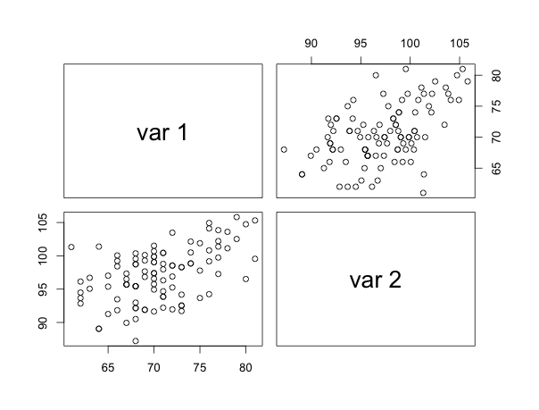
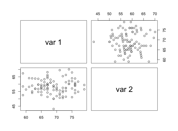
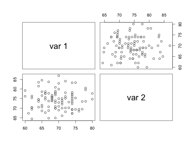
Notice how these plots show the pattern of the relationship between $x$ and $y$. In (a), we see the cloud of points tilted upwards and to the right; as the variable on the $x$ axis increases, so does the variable on the $y$ axis. In (b), we see the opposite; as the variable on the $x$ axis increases the variable on the $y$ axis decreases. The relationship isn’t that strong here so the pattern of the cloud tilted down and to the right is less obvious than in (c). In (c) it looks like a swarm of bees, all over the place, huddling in the middle, and with no pattern evident. This is no surprise because the two variables have an almost $0$ correlation. But scatter-plots alone don’t tell us whether a correlation is significant; a hypothesis test does. Given that $r$ is based on a sample it is estimating the true correlation between $x$ and $y$ in the population, denoted by $\rho$. One then needs to conduct a hypothesis test that will tell us whether in the population $\rho=0$ or $\rho \neq 0$.

\[\begin{array}{l} H_0: \rho=0 \\ H_A: \rho \neq 0 \end{array}\]

The test statistic is $t = \dfrac{r}{SE_r}$; where $SE_r = \sqrt{\dfrac{1-r^2}{n-2}}$ and as usual we reject $H_0$ if $p-value \leq \alpha$. We can also calculate asymptotic approximate confidence intervals for $\rho$ as

\[z - 1.96\sigma_z < \zeta < z + 1.96\sigma_z \text{ where } z=0.5ln\left( \dfrac{1+r}{1-r} \right)\]

where $\sigma_z = \sqrt{\dfrac{1}{n-3}}$ and $\zeta$ is the population analogue of the $z$ used to calculate confidence intervals. Because the $z$ involves the natural logarithm we back-transform via taking the antilog of the lower and upper bounds of the confidence interval.

Let us see scatter-plots and correlations in action with some real-world data to get a feel for patterns we might encounter.

Example 1

The Robert Wood Johnson Foundation’s County Health Rankings measure the health of nearly all counties in the nation and rank them within states. The Rankings are compiled using county-level measures from a variety of national and state data sources. The rankings employ a number of measures but those of interest and in use below are: (a) Premature Death (Years of potential life lost before age 75 per 100,000 population), (b) Adult Obesity (Percentage of adults that report a BMI of 30 or more), (c) Physical Inactivity (Percentage of adults aged 20 and over reporting no leisure-time physical activity ), (d) Uninsured (Percentage of population under age 65 without health insurance), (e) High School Graduation (Percentage of ninth-grade cohort that graduates in four years), and (f) Unemployment (Percentage of population ages 16 and older unemployed but seeking work).

If we look at all unique pairs of these variables, what should we expect? Well, I would expect premature death to be positively correlated with obesity, physical inactivity, uninsured, unemployment, and negatively correlated with high school graduation (under the belief that if you have $\geq$ high school education you are more likely to be employed, insured, etc).

Correlations in the County Health Rankings

FIGURE 11.2: Correlations in the County Health Rankings

I’ll setup a single pair of hypotheses so that you get the basic idea.

\[\begin{array}{l} H_0: \text{ Adult Obesity and Premature Death are not correlated } (\rho = 0) \\ H_1: \text{ Adult Obesity and Premature Death ARE correlated } (\rho \neq 0) \end{array}\]

As usual, we reject the null hypothesis if $p-value \leq \alpha$

In (a) and (b) we see a positive relationship with premature death increasing as adult obesity increases and uninsured rates increase, respectively. In (c), however, we see a negative relationship with premature death decreasing as high school graduation rates increase. The estimated correlation coefficients and $p-values$ are: (a) $r = 0.4966, p-value < 2.2e-16$, (b) $r = 0.3784, p-value < 2.2e-16$, and (c) $-0.1477, p-value = 1.055e-14$, with 95% confidence intervals of $0.4697, 0.5226$, $0.3480, 0.4081$, and $-0.1843, -0.1107$, respectively.

Example 2

Are care insurance premiums correlated with the percentage of drivers who were involved in fatal collisions and were speeding?

\[\begin{array}{l} H_0: \text{ Insurance premiums are not correlated with the percentage of drivers who were involved in fatal collisions and were speeding } (\rho = 0) \\ H_1: \text{ Insurance premiums ARE correlated with the percentage of drivers who were involved in fatal collisions and were speeding } (\rho \neq 0) \end{array}\]

FIGURE 11.3: Correlation between fatal collisions involving speeding and insurance premiums

The estimate correlation coefficient is $r=0.0425$, the $p-value = 0.7669$, and the 95% confidence interval is $(-0.2358, 0.3144$). Quite clearly we cannot reject the null; there is no correlation between the two metrics. You may have been surprised by these estimates since the plot may have lead you to expect a positive correlation. Well, a picture (and our a priori expectations) can always be at odds with the truth. Stereotypes, anyone??

11.1.1.1 Assumptions of the Pearson Correlation Coefficient

The Correlation Coefficient is based on the assumption of bivariate normality:

That $x$ and $y$ are each normally distributed – this assumption can be tested via the usual approaches to testing for normality. For our purposes, however, we will assume that normality holds.
That $x$ and $y$ are linearly related – the Pearson correlation coefficient applies to linear relationships so if $x$ and $y$ are non-linearly related the Pearson correlation coefficient should not be used.
That the cloud of points characterized by pairs of $x$ and $y$ has a circular or elliptical shape – this assumption can be visually checked.

If these assumptions are violated, we have some fallback solutions but those go beyond the purview of this course. We also will not worry about testing these assumptions for now.

11.1.2 Spearman Correlation Coefficient

While the Pearson correlation coefficient is designed for numeric variables, what if the measures are ordinal, such as states ranked by how healthy their populations are, counties ranked by the number of opioid deaths, or students ranked on the basis of their cumulative GPAs? Well, in these instances, where we have ordinal data, the Spearman correlation coefficient comes into use. Technically, the Spearman correlation coefficient measures the strength and association between the ranks of two variables assumed to be (i) randomly sampled, and (ii) with linearly related ranks. Again, we will not test these assumptions (since (i) is assumed to be true and testing (ii) is beyond our current scope). The mechanics are fairly simple:

Rank the scores of each variable separately, from low to high
Average the ranks in the presence of ties
Calculate $r_s=\dfrac{\sum \left(R - \bar{R} \right)\left( S - \bar{S}\right) }{\sum \left(R - \bar{R} \right)^2 \sum \left(S - \bar{S} \right)^2}$
$H_0$: $\rho_s = 0$; $H_1$: $\rho_s \neq 0$
Set $\alpha$
Reject $H_0$ if $P-value \leq \alpha$; Do not reject $H_0$ otherwise

Let us see a particularly interesting example.

11.1.2.1 Example 1

How reliable are witness accounts of “miracles?” One means of testing this is by comparing different accounts of extraordinary magic tricks. Of the many illusions performed by magicians, none is more renowned than the Indian rope trick. In brief, a magician tosses the end of a rope into the air and the rope forms a rigid pole. A boy climbs up the rope and disappears at the top. The magicians scolds the boy and asks him to return but with no response, and so climbs the rope himself, with a knife in hand, and does not return. The boy’s body falls in pieces from the sky into a basket on the ground. The magician then drops back to the ground and retrieves the boy from the basket, revealing him to be unharmed and in one piece.

Researchers tracked down 21 first-hand accounts and scored each narrative according to how impressive it was, on a scale of 1 to 5. The researchers also recorded the number of years that had lapsed between the date that the trick was witnessed and the date when the memory of the trick being performed was written down. Is there any association between the impressiveness of eyewitness accounts and the time lapsed since the account was penned?

FIGURE 11.4: The Indian rope trick

The figure is hard to read but it looks as if the more the years that have lapsed the higher the impressiveness score. The estimated correlation is $0.7843$ and has a $p-value = 2.571e-05$. The null hypothesis, of no correlation, is soundly rejected.

11.1.2.2 Example 2

You may have heard about the PISA Report every now and then when there are moans and groans about how the United States is performing academically compared to other Organization for Economic Cooperation and Development (OECD) nations. The report ranks countries in terms of students’ academic achievements and while it has its detractors (largely because of how the data are generated), PISA remains one of those obelisks policymakers and politicians can’t help but stare at even if they wished it would crumble into a mound of stand before next Monday. Well, if we look at how countries rank in terms of reading scores versus mathematics scores, what do we see? Are country ranks on these subjects correlated? Here is the scatter-plot:

FIGURE 11.5: PISA ranks on Reading and Mathematics

\[\begin{array}{l} H_0: \text{ Countries' ranks on reading and mathematics are not correlated } (\rho_s = 0) \\ H_1: \text{ Countries' ranks on reading and mathematics ARE correlated } (\rho_s \neq 0) \end{array}\]

Quite clearly, countries’ ranks on reading and mathematics are highly correlated. The estimated correlation is $r_s = 0.9374$ with a $p-value < 2.2e-16$, allowing us to easily reject the null hypothesis of no correlation.

11.2 Bivariate Regression

Do tall parents beget tall children? That was the question Sir Francis Galton grappled with questions of heredity, asking, among other things, whether parents pass on their traits to their offspring. What began as an inquiry with seeds turned into a study of the heights of children. What Galton realized was that regardless of parents’ average heights, children tended towards the average height of children of parents with a given height. In his own words, “It appeared from these experiments that the offspring did not tend to resemble their parents in size, but always to be more mediocre than they – to be smaller than the parents, if the parents were large; to be larger than the parents, if the parents were small.” This finding, since enshrined as the concept of regression to the mean, is the foundation of what we call regression analysis. We can explore Sir Galton’s point by examining the very data he worked with.

FIGURE 11.6: Sir Francis Galton’s data: Heights of parents and children

The scatter-plot emphasizes a few features of the data. First, there does seem to be an upward tilt to the cloud of data points, suggesting that on average as parents’ mid-height increases, so does the children’s height. In fact, the correlation is $r=0.4587$ with $p-value < 2.2e-16$, and so we can be confident that the two are indeed significantly and positively correlated. Second, every mid-height of the parents has children of multiple heights, rendering quite clearly the fact that there isn’t a $1:1$ relationship between parents’ average heights and children’s heights. Sometimes children are taller and other times they are shorter than their parents.

TABLE 11.1: Mean Child height per Parent height
Parent’s height	Mean Child height
64.0	65.3
64.5	65.4
65.5	66.7
66.5	67.1
67.5	67.6
68.5	68.0
69.5	68.7
70.5	69.6
71.5	70.1
72.5	71.9
73.0	73.0

What is the average height of the children for each parent mid-height? This is easily calculated, and has been tabulated for you below. The key point of this table is to illustrate the increasing average height of the child per increase in the parent mid-height. So when we encounter parents who have an average height of say 64 inches our best bet of their child’s height would be 65.3 inches, and so on. These mean heights of the children are plotted for you in the figure below. Notice that the line connecting these means is not a straight line.

FIGURE 11.7: Sir Francis Galton’s data: Heights of parents and children

What does any of this have to do with regression analysis? Everything. How? Because regression analysis revolves around trying to fit a straight line through a cloud of points representing pairs of values of two variables $x$ and $y$. The variable $y$ is what we will call our dependent variable and will be numeric and continuous while $x$ is out independent variable and can be either numeric or categorical. To aid our grasp of regression analysis we will restrict $x$ to be a numeric variable for the moment but relax this requirement down the road.

How could we fit a straight line through Galton’s data? By recalling the equation for a straight line: $y = m(x) + c$ where $m$ is the slope of the line and $c$ is in the intercept. Given two sets of coordinates $(x_1,y_1), (x_2,y_2)$, say $(-1,-1)$ and $(5, 1)$ respectively, we can calculate the slope of the straight line connecting these two points as $b = \dfrac{y_2 - y_1}{x_2 - x_1} = \dfrac{1 - (-1)}{5 - (-1)} = \dfrac{2}{6}=0.333$. This works for more than two data points as well, as shown below with a simple data-set.

TABLE 11.2: A small data-set for regression
x	y
-1	-1.000
0	-0.667
1	-0.333
2	0.000
3	0.333
4	0.667
5	1.000

Given these data, we can calculate the intercept $(a)$ by finding the value of $y$ when $x=0$. So one set of coordinates we want are $(0, y_0)$, and a second set picked arbitrarily could be $(5,1)$. Note that $y_0$ is the unknown value of the intercept $a$. Now, the slope is calculated for these pairs of points as

\[b = \dfrac{1 - y_0}{5 - 0}=\dfrac{1-y_0}{5}\]

Since we calculated the slope before we know the slope is 0.333, i.e., $b=0.333$. Substitute the value of the slope in the equation above and solve for the intercept $y_0$.

\[\begin{array}{l} b = \dfrac{1-y_0}{5} \\ 0.333 = \dfrac{1-y_0}{5} \\ \therefore 0.333 \times 5 = 1 - y_0 \\ \therefore (0.333 \times 5) - 1 = - y_0 \\ \therefore 1.665 - 1 = - y_0 \\ \text{multiply both sides of the equation to get rid of } -1 \text{ and rearrange}\\ \therefore y_0 = 1 - 1.665 = -0.665 \end{array}\]

We have both our slope and the intercept so we can write the equation for the straight line connecting the pairs of $(x,y)$ points as: $y = m(x) + c = 0.333(x) - 0.665$. Given this equation we can find the value of $y$ for any given value of $x$.

When $x=0$ $y = 0.333(0) - 0.665 = -0.665$
When $x=1$ $y = 0.333(1) - 0.665 = -0.332$
When $x=2$ $y = 0.333(2) - 0.665 = 0.001$
When $x=3$ $y = 0.333(3) - 0.665 = 0.334$
When $x=4$ $y = 0.333(4) - 0.665 = 0.667$
When $x=5$ $y = 0.333(5) - 0.665 = 1.000$

As $x$ increases by $1$, $y$ increases by $0.333$. That is the very definition for the slope of a straight line: The slope indicates how much $y$ changes by for a unit change in $x$. Unit change, in our case, will be treated as an increase of exactly $1$, so bear that in mind. Let us now plot these data points and draw the straight line we calculated through the cloud of points.

FIGURE 11.8: The regression line and cloud of points

In this case we have a single value of $y$ for a single value of $x$, unlike the Galton data where for each value of $x$ (parents’ average height) we had children of different heights $(y)$. What would the straight line look like in that case? Let us redraw the plot of parents’ and children’s heights with the straight line superimposed on the cloud of points.

FIGURE 11.9: Sir Francis Galton’s data: Heights of parents and children

Given the multiple $y$ values for each $x$ value we knew the straight line could not touch every point. Instead, it runs through the middle of the range of $x$ values for each $y$, except for the maximum value of $x$ where both points are well above the line. How close does this line come to the average of children’s heights calculated for each parent mid-height? Quite well, it turns out, except for the two highest values of parents’ mid-heights.

FIGURE 11.10: Sir Francis Galton’s data: Heights of parents and children

This demonstrates an important principle of the regression line: It will try to fit itself such that it minimizes the distance between itself and all the data points. Once it is fit, there is no way to rotate it up or down without making at least one data point farther away from the resulting line than was the case before. Hence the regression line is often also referred to as the line of best fit and the method of obtaining the estimates of the regression line as the method of ordinary least squares (OLS).

What if we used this line to predict a child’s height? Well, your prediction would be close to reality but the child could be taller or shorter than your predicted height. This drift we refer to as errors, and because these errors will occur, no matter how much we try to minimize them, we start writing the equation for the regression line as $y = \alpha + \beta(x) + \epsilon$ where $\alpha = intercept$, $\beta = slope$ and $\epsilon = errors$. In Galton’s data, the slope is estimated to be $0.6463$ and the intercept is $23.9415$, rendering the equation to be

\[\begin{array}{l} y = 23.9415 + 0.6463(x) \\ i.e., \text{ child's height } = 23.9415 + 0.6463(\text{ parents' mid-height }) \end{array}\]

The errors $(\epsilon)$ represent the drift between the actual $y_i$ value and the predicted value of y that is denoted as $\hat{y}_i$, i.e., $\epsilon_i = y_i - \hat{y}_i$. These errors reflect the fact that our regression line is either underestimating or overestimating actual $y$ values and so the amount of overestimation/underestimation is called the residuals – something left over by the regression line. For the estimated regression line, here are the $\hat{y}_i$ (the predicted values of $(y_i)$ and the residuals $(\hat{e}_i)$ for a snippet of the data.

TABLE 11.3: Predicted values and Residuals
Parent’s mid-height	Child’s height	Predicted Child’s height	Residual
64.0	61.7	65.3	-3.6
64.0	63.2	65.3	-2.1
64.0	63.2	65.3	-2.1
64.0	64.2	65.3	-1.1
64.0	64.2	65.3	-1.1
64.0	64.2	65.3	-1.1
64.0	64.2	65.3	-1.1
64.0	65.2	65.3	-0.1
64.0	66.2	65.3	0.9
64.0	66.2	65.3	0.9
64.0	67.2	65.3	1.9
64.0	67.2	65.3	1.9
64.0	68.2	65.3	2.9
64.0	69.2	65.3	3.9
64.5	61.7	65.6	-3.9
64.5	62.2	65.6	-3.4
64.5	63.2	65.6	-2.4
64.5	63.2	65.6	-2.4
64.5	63.2	65.6	-2.4
64.5	63.2	65.6	-2.4
64.5	64.2	65.6	-1.4
64.5	64.2	65.6	-1.4
64.5	64.2	65.6	-1.4
64.5	64.2	65.6	-1.4
64.5	65.2	65.6	-0.4
64.5	66.2	65.6	0.6
64.5	66.2	65.6	0.6
64.5	66.2	65.6	0.6
64.5	66.2	65.6	0.6
64.5	66.2	65.6	0.6

When $x = 64.0, \hat{y} = 65.3, y = 61.7$ and hence $\epsilon = 61.7 - 65.3 = -3.6$
When $x = 64.0, \hat{y} = 65.3, y = 63.2$ and hence $\epsilon = 63.2 - 65.3 = -2.1$
$\ldots$
When $x = 64.0, \hat{y} = 65.3, y = 65.2$ and hence $\epsilon = 65.2 - 65.3 = -0.1$
When $x = 64.0, \hat{y} = 65.3, y = 66.2$ and hence $\epsilon = 66.2 - 65.3 = 0.9$ 8 $\ldots$

The residual is the smallest when predicted $y$ and actual $y$ are close. If they were the same, the residual would be $0$. Now, what is the mean of $y$ when $x = 64.0$? This was $65.3$. So the predicted value of $y | x = 64.0$ is being calculated as the average height of all children born to parents with mid-heights of $64.0$ inches. This why the predicted value of a child’s height is always $65.3$ for these parents. In this sense, a predicted value from a regression is really a conditional mean prediction, conditional, that is, on the value of $x$. If you average all the residuals, they will be zero, i.e., $\bar{\epsilon = 0}$ and this is always true for any regression line.

Before we move on, note that the variance of the residuals is calculated as

\[\begin{array}{l} var(e_i) = \dfrac{\sum\left(e_i - \bar{e}\right)^2}{n-2} \\ = \dfrac{\sum\left(e_i - 0\right)^2}{n-2} \\ = \dfrac{\sum\left(e_i\right)^2}{n-2} \\ = \dfrac{\sum\left(y_i - \hat{y}_i\right)^2}{n-2} \end{array}\]

This is the $\dfrac{\text{ Sum of Squares of the Residuals}}{n-2} = \text{Mean of the Sum of Squares of the Residuals} = MS_{residual}$. This is the average prediction error in squared units so if we take the square-root, we get the average prediction error $RMSE = \sqrt{\text{Mean of the Sum of Squares of the Residuals}}$. The smaller is this value, the better is the regression line fitting the data.

11.2.1 The Method of Ordinary Least Squares

The method of ordinary least squares estimates the slope and the intercept by looking to minimize the sum of squared errors (SSE), i.e., $\sum(e_i)^2 = \sum\left(y_i - \hat{y}_i\right)^2$ with the slope estimated as $\hat{\beta} = \dfrac{\sum\left(x_i - \bar{x}\right)\left(y_i - \bar{y}\right)}{\sum\left(x_i - \bar{x}\right)^2}$. Once $\hat{\beta}$ is estimated, the intercept can be calculated via $\hat{\alpha} = \bar{y} - \hat{\beta}\left(\bar{x}\right)$. The standard error of the slope is $s.e._{\hat{\beta}} = \sqrt{ \dfrac{\text{Mean of the Sum of Squares of the Residuals}}{\sum\left(x_i - \bar{x}\right)^2} }$.

11.2.2 Population Regression Function vs. Sample Regression Function

Now, assume that the Galton data represent the population and instead of working with the population data you have a random sample to work with. Below I have drawn four random samples, each with $100$ data points randomly selected from the Galton data-set, estimated the regression line and then plotted the cloud of points plus the regression line. What do you see as you scan the four plots?

FIGURE 11.11: Four random samples from Galton’s data

Note that each sample yields different estimates as compared to the population regression line where the regression equation was $23.94 + 0.64(x)$. This is to be expected since a sample will approximate the population but rarely be identical. Because we are dealing with a sample, we distinguish between the population regression line and the sample regression line by writing the latter as $y = a + b(x) + e$.

11.2.3 Hypotheses

Of course, we need to assess both the statistical significance of our sample regression line, and how well the line fits the data. Let us look at the hypothesis tests first. We have estimated two quantities – the intercept and the slope – and hence will have two hypothesis tests.

\[\begin{array}{l} H_0: \alpha = 0 \\ H_1: \alpha \neq 0 \end{array}\]

and

\[\begin{array}{l} H_0: \beta = 0 \\ H_1: \beta \neq 0 \end{array}\]

The test statistic for each relies on the standard errors of $a$ and $b$. In particular, the test statistic for the slope is $t_{\hat{b}} = \dfrac{\hat{b}}{s.e._{\hat{b}}}$ and if the $p-value \leq \alpha$ we reject the null that $\beta = 0$. Likewise, for the intercept we have $s.e._{\hat{a}} = \sqrt{MS_{residual}}\left(\sqrt{\dfrac{\sum x_i^2}{n\sum\left(x_i - \bar{x}\right)^2}} \right)$, leading to $t_{\hat{a}} = \dfrac{\hat{a}}{s.e._{\hat{a}}}$. We can also estimate the confidence interval estimates for $\hat{a}$ and $\hat{b}$ to get a sense of the intervals within which $\alpha$ and $\beta$ are likely to fall (in the population).

11.2.4 The $R^2$

In addition to the RMSE, the average prediction error, we also rely on the $R^2$, which tells us what percent of the variation in $y$ can be explained by the regression model. How is this calculated? Well, we already calculated the sum of squares for the residuals (SSE), which was $\sum \left(y_i - \bar{y}\right)^2$. Now, we do know that the total variation in $y$ can be calculated as $\sum\left(y_i - \bar{y}\right)^2$, so let us label this SST. The total variation in $y$ has to be made up of the SSE and the amount of variation being captured by the regression. Let us label this latter quantity SSR, and note that it can be calculated as $SSR = \sum\left(\hat{y}_i - \bar{y}\right)^2$. Since $SST = SSR + SSE$, we can assess what proportion of variance in $y$ is explained by the regression by calculating $\dfrac{SSR}{SST} \ldots$ which is the $R^2$.

If the regression model is terrible, $R^2 \to 0$ and if the regression model is excellent, $R^2 \to 1$. That is, $0 \leq R^2 \leq 1$ … the $R^2$ will lie in the $\left[0, 1\right]$ interval. In practice, we adjust the $R^2$ for the number of independent variables used and rely on this adjusted $R^2$, denoted as $\bar{R}^2$, and calculated as $\bar{R}^2 = 1 - \left(1 - R^2\right)\left(\dfrac{n-1}{n-k-1}\right)$ where $k =$ the number of independent variables being used.

11.2.5 Confidence Intervals vs. Prediction Intervals

Technically speaking, $\hat{y}_{i}$ is a point estimate for $y_{i}$ because it is a single estimate and tells us nothing about the interval within which the predicted value might fall. Confidence intervals and Prediction intervals, however, do, but they are not the same thing. Specifically, while the confidence interval is an interval estimate of the mean value of y for a specific value of $x$, the prediction interval is an interval estimate of the predicted value of y for a specific value of $x$.

Given $x_{p} =$ specific value of $x$ and $y_{p} =$ specific value of $y$ for $x = x_{p}$, $E(y_{p}) =$ expected value of $y$ given $x = x_{p}$ is defined as $\hat{y}_{p} = \hat{a} + \hat{b}(x_{p})$. The variance is, in turn, given by var($\hat{y}_{p}$) $= s^{2}_{\hat{y}_{p}} = s^{2}\left[\dfrac{1}{n} + \dfrac{(x_{p} - \bar{x})^{2}}{\sum(x_{i} - \bar{x})^{2}}\right]$, which leads to s($\hat{y}_{p}$) $= s_{\hat{y}_{p}}=s\sqrt{\left[\dfrac{1}{n} + \dfrac{(x_{p} - \bar{x})^{2}}{\sum(x_{i} - \bar{x})^{2}} \right]}$

Now, the confidence interval is given by $\hat{y}_{p} \pm t_{\alpha/2}\left(s_{\hat{y}_p}\right)$. Every time we calculate this interval we know we could be wrong on two counts – $b_{0}; b_{1}$. Fair enough, since both have been estimated from the data and could be wrong.

However, if we want to predict $y$ for some $x$ value not in the sample, we know here we could be wrong on three counts – $b_{0}; b_{1}; \text{ and } e$. This forces an adjustment in the variance calculated earlier to now be defined as $s^{2}_{ind} = s^{2} + s^{2}_{\hat{y}_{p}}$, where $s^{2}_{ind} = s^{2} + s^{2}\left[\dfrac{1}{n} + \dfrac{(x_{p} - \bar{x})^{2}}{\sum(x_{i} - \bar{x})^{2}}\right] = s^{2} \left[1 + \dfrac{1}{n} + \dfrac{(x_{p} - \bar{x})^{2}}{\sum(x_{i} - \bar{x})^{2}}\right]$ and hence $s_{ind} = s\sqrt{\left[1 + \dfrac{1}{n} + \dfrac{(x_{p} - \bar{x})^{2}}{\sum(x_{i} - \bar{x})^{2}}\right]}$. The prediction interval is then calculated as $\hat{y}_{p} \pm t_{\alpha/2}\left(s_{ind}\right)$

With the Galton data, this is what the scatter-plot would look like with the confidence intervals and predictions intervals added to the regression line. Focus on these intervals.

FIGURE 11.12: Confidence vs. Prediction Intervals

Notice how much wider the prediction intervals are (the red dashed lines); this is because we have made an adjustment for the additional uncertainty surrounding an individual prediction. Notice also that the confidence intervals flex inward, toward the regression line, in the center of the distribution but then flew outward at either extreme of the regression line. This is a result of the fact that the regression estimates are built around $\bar{x}$ and $\bar{y}$ and hence the greatest precision we have is when we are predicting $y$ for $\bar{x}$, i.e., when predicting $\hat{y}_{\bar{x}} = \hat{a} + \hat{b}\left(\bar{x}\right)$.

To sum up our discussion of interval estimates, remember that the confidence interval is in use when predicting the average value of $y$ for a specific value of $x$. However, when we are predicting a specific value of $y$ for a given $x$, then the prediction interval comes into use. Further, confidence intervals will hug the regression line most closely around $\bar{x}$, and widen as you progressively move towards $x_{min}$ and $x_{max}$.

11.2.5.1 Example 1

	child
Predictors	Estimates	CI	p
(Intercept)	30.50	13.42 – 47.59	0.001
parent	0.55	0.30 – 0.80	<0.001
Observations	100
R² / R² adjusted	0.161 / 0.153

With a random sample drawn from the Galton data-set, can we claim that parents’ mid-heights predict the child’s height? If they do, how good is the fit of the model? It turns out that the intercept was estimated as $\hat{a} = 21.1143$ and has a $p-value = 0.00921$ while the slope was estimated as $0.6913$ and has a $p-value = 4.49e-08$. So both the intercept and the slope are statistically significant. The $RMSE = 2.216$ and the $\bar{R}^2 = 0.2568$.

When the parents’ mid-height is $=0$ the child’s height is predicted to be $21.11$ inches
As parents’ mid-height increases by $1$, the child’s height increases by 0.6913 inches
If we used this regression model to predict a child’s height, on average our prediction error would be $2.216$ inches, i.e., we would overpredict or underpredict the child’s actual height by $\pm 2.216$ inches
The $\bar{R}^2 = 0.2568$, indicating that about $25.68\%$ of the variation in the child’s height can be explained by this regression model (i.e., by using the parents’ mid-height as an independent variable)
The 95% confidence interval around $\hat{a}$ is $\left[5.34, 36.88\right]$, indicating that we can be about 95% confident that the population intercept lies in the $\left[5.34, 36.88\right]$ range
The 95% confidence interval around $\hat{b}$ is $\left[0.46, 0.92\right]$, indicating that we can be about 95% confident that the population slope lies in the $\left[0.46, 0.92\right]$ range

Note that the intercept will not always make sense from a real-world perspective, i.e., you can’t have parents’ mid-height be $0$ since that would mean there are no parents! However, we retain the intercept for mathematical necessity but accommodate for the often nonsensical meaning of the intercept by not interpreting it all. It is needed for the mathematics to work out but need not be interpreted. Note also that since we are only explaining about $25.68\%$ of the variation in children’s heights, there is $100 - 25.68 = 74.32\%$ of the variation left to be explained. Maybe there are other independent variables we could have used that would do a better job of predicting the child’s height as in, for example, nutrition, physical activity, good health care during the child’s early years, and so on.

11.2.5.2 Example 2

Let us revisit the question of premature death and adult obesity. How well can we predict premature death from adult obesity? Since the original data we looked at included all counties in the U.S., I will draw a random sample of 100 counties to fit the regression model.

	Premature Death
Predictors	Estimates	CI	p
(Intercept)	0.94	0.79 – 1.10	<0.001
Adult Obesity	0.00	-0.01 – 0.01	0.626
Observations	99
R² / R² adjusted	0.002 / -0.008

The intercept is $-28.83$ but is not statistically significant since the $p-value = 0.988$
The slope is $264.78$ and is statistically significant given the $p-value = -1.77e-05$, indicating that as the percent of obese adults increases by $1$, the number of premature deaths increases by about 265.
The $\bar{R}^2 = 0.1652$, indicating that we can explain about $16.52\%$ of the variation in premature deaths with this regression model.
The $RMSE = 2355.516$, indicating that average prediction error would be $\pm 2355.516$ if this model were used. Note the high value here, indicative of a sizable prediction error. Being off the truth by $2355$ premature deaths is a lot!

Here are the data with the scatter-plot, regression line, and confidence intervals. Note that the regression equation superimposed on the plot has estimates rounded up; hence the marginal difference between these and the estimates interpreted above. Note also that the $R^2$ is being reported, not $\bar{R}^2$.

FIGURE 11.13: Predicting Premature Death from Adult Obesity

11.2.6 Dummy Variables

In the examples so far we have worked with numeric variables – parents’ mid-height, adult obesity, and so on. However, what if we had categorical variables and wanted to examine, for example, if premature deaths vary across males and females? If public school district performance differs between Appalachian and non-Appalachian Ohio? Do carbon dioxide $CO_2$ emissions vary between the developed and the developing countries? These types on interesting questions lend themselves to regression analysis rather easily. To see how these models are fit and interpreted, let us work with a specific example. The data I will utilize span the 50 states and Washington DC for the 1977-1999 period, with information on the following variables:

state = factor indicating state.
year = factor indicating year.
violent = violent crime rate (incidents per 100,000 members of the population).
murder = murder rate (incidents per 100,000).
robbery = robbery rate (incidents per 100,000).
prisoners = incarceration rate in the state in the previous year (sentenced prisoners per 100,000 residents; value for the previous year).
afam = percent of state population that is African-American, ages 10 to 64.
cauc = percent of state population that is Caucasian, ages 10 to 64.
male = percent of state population that is male, ages 10 to 29.
population = state population, in millions of people.
income = real per capita personal income in the state (US dollars).
density = population per square mile of land area, divided by 1,000.
law = factor. Does the state have a shall carry law in effect in that year? If the value is “yes,” then the state allows individuals to carry a concealed handgun provided they meet certain criteria.

To keep things simple let us shrink this data-set to the year 1999. The substantive question of interest is: Do concealed carry permits reduce robberies?

\[\begin{array}{l} H_0: \text{ Concealed carry laws have no impact on robbery rates } (\beta = 0) \\ H_1: \text{ Concealed carry laws have an impact on robbery rates } (\beta \neq 0) \end{array}\]

The regression model that could be used would assume the following structure: $\hat{y} = \hat{a} + \hat{b}\left(law\right) + \hat{e}$. The variable “law” is a categorical variable that assumes two values – $x = 1$ indicates the state allows concealed carry and $x = 0$ indicates that the state does not allow concealed carry. What will the regression equation look like if $x=1$ versus $x=0$?

\[\begin{array}{l} \hat{y} = \hat{a} + \hat{b}\left(x \right) \\ \text{When } x = 1: \hat{y} = \hat{a} + \hat{b}\left(1\right) = \hat{a} + \hat{b} \\ \text{When } x = 0: \hat{y} = \hat{a} + \hat{b}\left(0\right) = \hat{a} \end{array}\]

Aha! The predicted value of $y$ for states with no concealed carry laws is just the estimated intercept while the predicted value of $y$ for states with concealed carry laws is the estimated intercept $+$ the estimated slope. This tells us that difference in robbery rates between states with and without concealed carry laws is just the estimated slope $\hat{b}$. Now on to visualizing the data and then to fitting the regression model.

FIGURE 11.14: Box-plots of Robbery rates by Law

	robbery
Predictors	Estimates	std. Error	std. Beta	standardized std. Error	CI	standardized CI	Statistic	p
(Intercept)	155.09	20.33	0.34	0.21	114.23 – 195.94	-0.07 – 0.75	7.63	<0.001
law [yes]	-59.59	26.96	-0.60	0.27	-113.77 – -5.40	-1.15 – -0.05	-2.21	0.032
Observations	51
R² / R² adjusted	0.091 / 0.072

The box-plots show an outlier for law = “no” and a higher median robbery rate for the “no” group versus the “yes” group; seemingly, states without concealed carry laws have on average higher robbery rates.

The estimated regression line is $\hat{y} = 155.09 -59.59\left(law\right)$. That is, states without a law are predicted to have about $114$ robberies per 100,000 persons. States with a law, on the other hand, are predicted to have almost 114 fewer robberies per 100,000 persons. Note that both the intercept and the slope are statistically significant, the $RMSE = 95.36$ and the $\bar{R}^2 = 0.0720 = 7.20\%$.

Wait a minute. What about that outlier we see in the box-plot? Couldn’t that be influencing our regression estimates? Let us check by dropping that data point and re-estimating the regression model.

FIGURE 11.15: Box-plots of Robbery rates by Law (no outlier)

	robbery
Predictors	Estimates	std. Error	std. Beta	standardized std. Error	CI	standardized CI	Statistic	p
(Intercept)	131.79	13.90	0.32	0.21	103.83 – 159.75	-0.11 – 0.75	9.48	<0.001
law [yes]	-36.29	18.26	-0.55	0.28	-73.00 – 0.42	-1.11 – 0.01	-1.99	0.053
Observations	50
R² / R² adjusted	0.076 / 0.057

Now, the estimated intercept is $131.79$ and statistically significant. The estimated slope is $-36.29$ and has a $p-value = 0.0526$, and so it is not statistically significant! In brief, without the outlier, average robbery rates per 100,000 persons do not appear to differ between states with/without concealed carry laws. What is the moral of the story? Regression estimates will be influenced by outliers, the more extreme the outlier, the more the influence.

The preceding example involved a two-category variable. What if the variable had three or more categories? What would the regression model look like and how would we interpret the results? Assume, for example, that we are interested in looking at the wages of men who had an annual income greater than USD 50 in 1992 and were neither self-employed nor working without pay. The sample spans men aged 18 to 70 and is drawn from the March 1988 Current Population Survey. The data-set includes the following variables:

wage = Wage (in dollars per week).
education = Number of years of education.
experience = Number of years of potential work experience.
ethnicity = Factor with levels “cauc” and “afam” (African-American).
smsa = Factor. Does the individual reside in a Standard Metropolitan Statistical Area (SMSA)?
region = Factor with levels “northeast,” “midwest,” “south,” “west.”
parttime = Factor. Does the individual work part-time?

The question of interest here will be whether wages differ by Census regions.

\[\begin{array}{l} H_0: \text{ Wages do not differ by Census regions } \\ H_1: \text{ Wages do differ by Census regions } \end{array}\]

The variable “region” is coded as follows: $\text{Northeast}: x=1$, $\text{Midwest}: x=2$, $\text{South}: x=3$, $\text{West}: x=4$. The usual regression equation would be $\hat{y} = \hat{a} + \hat{b}\left(x\right)$. However, with categorical variables representing some attribute that has more than 2 categories we write the regression equation in a different manner. Specifically, we create a dummy variable for each of mutually exclusive categories as follows:

\[\begin{array}{l} \text{Northeast}: = 1 \text{ if in the Northeast }; 0 \text{ otherwise (i.e., if in the Midwest, South, West)} \\ \text{Midwest}: = 1 \text{ if in the Midwest }; 0 \text{ otherwise (i.e., if in the Northeast, South, West)} \\ \text{South}: = 1 \text{ if in the South }; 0 \text{ otherwise (i.e., if in the Northeast, Midwest, West)} \\ \text{West}: = 1 \text{ if in the West }; 0 \text{ otherwise (i.e., if in the Northeast, Midwest, South)} \end{array}\]

This leads to the regression equation being $\hat{y} = \hat{a} + \hat{b}_1\left(Northeast\right) + \hat{b}_2\left(Midwest\right) + \hat{b}_3\left(South\right) + \hat{b}_4\left(West\right)$ but in estimating the regression model we only use three of the dummy variables. This is a general rule: With a categorical variable that results in $k$ dummy variables only $k-1$ dummy variables should be included in the model unless the intercept is excluded. How do we decide which region to leave out? The rule of thumb is to leave out the modal category (i.e., the category that has the highest frequency).

TABLE 11.4: Frequency Table for Census Regions
Census Region	Frequency
northeast	6441
midwest	6863
south	8760
west	6091

In this data-set, the modal category happens to be the South and so we will estimate the model as $\hat{y} = \hat{a} + \hat{b}_1\left(Northeast\right) + \hat{b}_2\left(Midwest\right) + \hat{b}_3\left(West\right)$. Now we break this down so we know how to interpret the estimates of $\hat{y}$:

\[\begin{array}{l} \text{In the Northeast}: \hat{y} = \hat{a} + \hat{b}_1\left(Northeast\right) + \hat{b}_2\left(Midwest\right) + \hat{b}_3\left(West\right) = \hat{a} + \hat{b}_1\left(1\right) + \hat{b}_2\left(0\right) + \hat{b}_3\left(0\right) = \hat{a} + \hat{b}_1 \\ \text{In the Midwest}: \hat{y} = \hat{a} + \hat{b}_1\left(Northeast\right) + \hat{b}_2\left(Midwest\right) + \hat{b}_3\left(West\right) = \hat{a} + \hat{b}_1\left(0\right) + \hat{b}_2\left(1\right) + \hat{b}_3\left(0\right) = \hat{a} + \hat{b}_2 \\ \text{In the West}: \hat{y} = \hat{a} + \hat{b}_1\left(Northeast\right) + \hat{b}_2\left(Midwest\right) + \hat{b}_3\left(West\right) = \hat{a} + \hat{b}_1\left(0\right) + \hat{b}_2\left(0\right) + \hat{b}_3\left(1\right) = \hat{a} + \hat{b}_3 \\ \text{In the South}: \hat{y} = \hat{a} + \hat{b}_1\left(Northeast\right) + \hat{b}_2\left(Midwest\right) + \hat{b}_3\left(West\right) = \hat{a} + \hat{b}_1\left(0\right) + \hat{b}_2\left(0\right) + \hat{b}_3\left(0\right) = \hat{a} \end{array}\]

Aha! Since we excluded South the, intercept $(\hat{a})$ reflects the impact of being in the South. Keeping this in mind, let us see how to interpret the rest of the regression estimates shows in the regression equation below:

	wage
Predictors	Estimates	std. Error	std. Beta	standardized std. Error	CI	standardized CI	Statistic	p
(Intercept)	558.31	4.83	-0.10	0.01	548.84 – 567.78	-0.12 – -0.08	115.56	<0.001
region [northeast]	95.73	7.42	0.21	0.02	81.18 – 110.28	0.18 – 0.24	12.90	<0.001
region [midwest]	46.37	7.29	0.10	0.02	32.08 – 60.66	0.07 – 0.13	6.36	<0.001
region [west]	56.46	7.54	0.12	0.02	41.68 – 71.25	0.09 – 0.16	7.48	<0.001
Observations	28155
R² / R² adjusted	0.006 / 0.006

\[\begin{array}{l} \hat{y} = \hat{a} + \hat{b}_1\left(Northeast\right) + \hat{b}_2\left(Midwest\right) + \hat{b}_3\left(West\right) \\ \hat{y} = 558.308 + 95.731\left(Northeast\right) + 46.371\left(Midwest\right) + 56.463\left(West\right) \end{array}\]

Predicted average wage in the Northeast is $558.308 + 95.731 = 654.039$
Predicted average wage in the Midwest is $558.308 + 46.371 = 604.679$
Predicted average wage in the Northeast is $558.308 + 56.463 = 614.771$
Predicted average wage in the South is $558.308$

The $p-values$ are basically $0$ for the intercept and the the three dummy variables and hence these results suggest that region does matter; wages differ by Census region, with those in the Northeast having the highest average wage, followed by the Northeast, then the Midwest, and finally the West. In closing, the $RMSE = 452.2$ and the $\bar{R}^2 = 0.005959 = 0.5959\%$. Clearly this is a terrible regression model because we are hardly explaining any of the variation in wages.

11.3 Multiple Regression

Thus far we have restricted out attention to a single independent variable, largely because it is easier to understand the logic of regression analysis with a single independent variable. However, few things, if any, can be explained by looking at a single independent variable. Instead, we often have to include multiple independent variables because the phenomenon the dependent variable represents is extremely complex. For example, think about trying to predict stock prices, climate change, election results, students’ academic performance, health outcomes, and so on. None of these are easy phenomenon to comprehend, leave alone capture via a single independent variable. Consequently, we now turn to the more interesting world of multiple regression analysis We will start with at least two independent variables, each of which may be numeric or categorical. For ease of comprehension I’ll stick with the wage data-set.

Say we have two independent variables, $x_1$ and $x_2$. Now the regression equation is specified as

\[\hat{y} = \hat{a} + \hat{b}_1\left( x_1 \right) + \hat{b}_2\left( x_2 \right)\]

With three independent variables the equation becomes

\[\hat{y} = \hat{a} + \hat{b}_1\left( x_1 \right) + \hat{b}_2\left( x_2 \right) + \hat{b}_3\left( x_3 \right)\]

and so on.

Now the way we interpret $\hat{a}, \hat{b}_1, \hat{b}_2, \text{ and } \hat{b}_3$ changes. Specifically,

$\hat{a}$ is the predicted value of $y$ when all independent variables are $=0$
$\hat{b}_1$ is the partial slope coefficient on $x_1$ and indicates the change in $y$ for a unit change in $x_1$ holding all other independent variables constant
$\hat{b}_2$ is the partial slope coefficient on $x_2$ and indicates the change in $y$ for a unit change in $x_2$ holding all other independent variables constant
$\hat{b}_3$ is the partial slope coefficient on $x_3$ and indicates the change in $y$ for a unit change in $x_3$ holding all other independent variables constant
and so on

The interpretation of the $RMSE$ and $\bar{R}^2$ remains the same. Hypotheses are setup for each independent variable as usual. Generating predicted values requires some work though because you have to set each independent variable to a specific value when generating $\hat{y}$. We typically start by setting all independent variables to their mean (or median) value (if the independent variable is numeric) and to their modal values (if the independent variable is categorical). Let us anchor our grasp of these in the context of a specific problem.

11.3.1 Two Numeric (i.e., Continuous) Independent Variables

Say we are interested in studying the impact of two continuous independent variables, education and experience, on wage, i.e., $\hat{y} = \hat{a} + \hat{b}_1\left( education \right) + \hat{b}_2\left( experience \right)$. When you fit this regression model the estimates will be as follows:

	wage
Predictors	Estimates	std. Error	std. Beta	standardized std. Error	CI	standardized CI	Statistic	p
(Intercept)	-385.08	13.24	0.00	0.01	-411.04 – -359.13	-0.01 – 0.01	-29.08	<0.001
education	60.90	0.88	0.39	0.01	59.17 – 62.63	0.38 – 0.40	68.98	<0.001
experience	10.61	0.20	0.31	0.01	10.22 – 10.99	0.29 – 0.32	54.19	<0.001
Observations	28155
R² / R² adjusted	0.177 / 0.177

The intercept is statistically significant and is $\hat{a} = -385.0834$, indicating that when both education and experience are $=0$, predicted wage is $-385.0834$. Note that this makes no substantive sense but we are not interested in interpreting the intercept per se.
The partial slope on education is statistically significant and is $\hat{b}_1 = 60.8964$, indicating that holding experience constant, for every one more year of education wage increases by $60.8964.
The partial slope on experience is statistically significant and is $\hat{b}_2 = 10.6057$, indicating that holding education constant, for every one more year of experience wage increases by $10.6057.
$RMSE = 411.5$, indicating that average prediction error from this regression model would be $\pm 411.5$
The $\bar{R}^2 = 0.1768$ indicating that about $17.68\%$ of the variation in wage is explained by this regression model.

What about predicted values? Let us calculate a few.

Predict wage when education is at its mean and experience is at its mean:

\[\begin{array}{l} = -385.0834 + 60.8964(education) + 10.6057(experience) \\ = -385.0834 + 60.8964(13.06787) + 10.6057(18.19993) \\ = -385.0834 + 795.7862 + 193.023 = 603.7258 \end{array}\]

Predict wage when education is at its mean and experience is (i) $8$, and (ii) $27$:

\[\begin{array}{l} = -385.0834 + 60.8964(13.06787) + 10.6057(8) \\ = -385.0834 + 795.7862 + 84.8456 = 495.5484 \end{array}\]

\[\begin{array}{l} = -385.0834 + 60.8964(13.06787) + 10.6057(27) \\ = -385.0834 + 795.7862 + 286.3539 = 697.0567 \end{array}\]

Predict wage when experience is at its mean and education is (i) $12$, and (ii) $15$:

\[\begin{array}{l} = -385.0834 + 60.8964(12) + 10.6057(18.19993) \\ = -385.0834 + 730.7568 + 193.023 = 538.6964 \end{array}\]

\[\begin{array}{l} = -385.0834 + 60.8964(15) + 10.6057(18.19993) \\ = -385.0834 + 913.446 + 193.023 = 721.3856 \end{array}\]

11.3.2 One Numeric and One Categorical Independent Variable

Let us stay with education as the continuous independent variable but add a categorical independent variable – parttime – that tells us whether the individual was working full-time $(parttime = 0)$ or not $(parttime = 1)$. The regression model is:

\[wage = \hat{\alpha} + \hat{\beta_1}(education) + \hat{\beta_2}(parttime) + e\]

	wage
Predictors	Estimates	std. Error	std. Beta	standardized std. Error	CI	standardized CI	Statistic	p
(Intercept)	27.99	11.50	0.08	0.01	5.44 – 50.54	0.07 – 0.09	2.43	0.015
education	46.82	0.86	0.30	0.01	45.14 – 48.49	0.29 – 0.31	54.63	<0.001
parttime [yes]	-402.05	8.70	-0.89	0.02	-419.10 – -385.00	-0.92 – -0.85	-46.22	<0.001
Observations	28155
R² / R² adjusted	0.155 / 0.155

As estimated, the model turns out to be:

\[wage = 27.9930 + 46.8153(education) - 402.0493(parttime)\]

and this regression equation makes clear that the estimate of $-402.0493$ applies to the case of a part-time employee. What would predicted values look like for part-time versus full-time employees, for specific values of education.

For a part-time employee, predicted wage is $= 27.9930 + 46.8153(education) - 402.0493(1) = -374.0563 + 46.8153(education)$
For a full-time employee, predicted wage is $= 27.9930 + 46.8153(education) - 402.0493(0) = 27.9930 + 46.8153(education)$

So quite clearly, holding all else constant, on average, part-time employees make $402.0493$ less than full-time employees. For every one more year of education, wage increases by $46.8153$. When $education = 0$ and the employee is a full-time employee, predicted wage is $27.9930$.

Now we switch things up by fitting a regression model that predicts wage on the basis of two categorical variables. We have already worked with parttime so let us add the second categorical variable, region. The resulting regression model is:

\[wage = \hat{\alpha} + \hat{\beta_1}(parttime) + \hat{\beta_2}(region) + e\]

When you estimate the model you will see the following results:

	wage
Predictors	Estimates	std. Error	std. Beta	standardized std. Error	CI	standardized CI	Statistic	p
(Intercept)	593.92	4.74	-0.02	0.01	584.63 – 603.21	-0.04 – -0.00	125.34	<0.001
parttime [yes]	-405.68	9.12	-0.89	0.02	-423.57 – -387.80	-0.93 – -0.86	-44.47	<0.001
region [northeast]	91.11	7.18	0.20	0.02	77.04 – 105.17	0.17 – 0.23	12.70	<0.001
region [midwest]	48.41	7.05	0.11	0.02	34.60 – 62.22	0.08 – 0.14	6.87	<0.001
region [west]	62.54	7.29	0.14	0.02	48.25 – 76.84	0.11 – 0.17	8.58	<0.001
Observations	28155
R² / R² adjusted	0.071 / 0.071

that then lead to the following regression equation:

\[wage = 593.921 - 405.684(parttime = yes) + 91.106(region = northeast) + 48.412(region = midwest) + 62.544(region = west)\]

The correct starting point would be to see what the Intercept represents. Since we see a partial slope for parttime = yes the Intercept must be absorbing parttime = no, and the omitted region = south. That is, the Intercept is yielding the predicted wage $(593.921)$ when the individual is a full-time employee who lives in the South. Let us spell out this situation and all other possibilities as well.

Full-time living in the South: $wage = 593.921$
Full-time living in the Northeast: $wage = 593.921 + 91.106 = 685.027$
Full-time living in the Midwest: $wage = 593.921 + 48.412 = 642.333$
Full-time living in the West: $wage = 593.921 + 62.544 = 656.465$
Part-time living in the South: $wage = 593.921 - 405.684 = 188.237$
Full-time living in the Northeast: $wage = 593.921 + 91.106 - 405.684 = 279.343$
Full-time living in the Midwest: $wage = 593.921 + 48.412 - 405.684 = 236.649$
Full-time living in the West: $wage = 593.921 + 62.544 - 405.684 = 250.781$

11.3.3 Interaction Effects

Say we are back in the world of the regression model with education and parttime. When we fit this model before, we saw a constant difference in predicted wage for the employee’s full-time/part-time status. In particular, we saw predicted wage being lower by a constant amount for every level of education. However, what if part-time/full-time status has more of an impact on wage at low education levels than it does at high education levels? This is quite likely to be true if, once you have sufficient education, part-time status does not depress your wage as much as it does when you have low educational attainment. Situations such as these are referred to as interaction effects. In general, An interaction effect exists when the magnitude of the effect of one independent variable $(x_1)$ on a dependent variable $(y)$ varies as a function of a second independent variable $(x_2)$. Models such as these are written as follows:

\[wage = \hat{\alpha} + \hat{\beta_1}(education) + \hat{\beta_2}(parttime) + \hat{\beta_3}(education \times parttime) + e\]

Now, we may either have a priori expectations of an interaction effect or just be looking to see if an interaction effect exists. Regardless, if we were to fit such a model to the data, we would see the following:

	wage
Predictors	Estimates	std. Error	std. Beta	standardized std. Error	CI	standardized CI	Statistic	std. Statistic	p	std. p
(Intercept)	-19.07	11.97	0.08	0.01	-42.53 – 4.39	0.07 – 0.09	-1.59	13.87	0.111	<0.001
education	50.41	0.89	0.32	0.01	48.66 – 52.17	0.31 – 0.33	56.41	56.41	<0.001	<0.001
parttime [yes]	137.35	40.38	-0.89	0.02	58.21 – 216.49	-0.93 – -0.86	3.40	-46.73	0.001	<0.001
education * parttime [yes]	-41.52	3.04	-0.27	0.02	-47.47 – -35.57	-0.30 – -0.23	-13.68	-13.68	<0.001	<0.001
Observations	28155
R² / R² adjusted	0.161 / 0.161

Note the estimated regression line:

\[wage = - 19.0698 + 50.4144(education) + 137.3511(parttime) - 41.5221(education \times parttime)\]

For a model such as this, we speak of two types of effects – (a) a main effect of an independent variable, and an (b) interaction effect for each variable. These effects are best understood visually, and then through a series of calculations that will underline what is going on in the model.

FIGURE 11.16: Interaction between parttime and education

You see two regression lines, one for part-time employees and the other for full-time employees, each drawn for specific values of education. At low education levels, full-time employees $(parttime = no)$ have a lower average wage than do part-time employees $(parttime = yes)$. At a certain education level there seems to be no difference at all, roughly around $education = 3$. Once the employee has 4 or more years of education, however, the gap in wages increases in favor of full-time employees for each additional year of education. This widening gap is clearly visible in the steepening regression line for $parttime = no$ at higher education levels. We could also calculate predicted wage when $education = 0$, and then for $education = 3$, and then for $education = 18$ to see the gap in action. Let us do so now.

For a part-time employee with $0$ years of education, the predicted wage is

\[\begin{array}{l} wage = - 19.0698 + 50.4144(education = 0) + 137.3511(parttime = 1) - 41.5221(0 \times 1) \\ = - 19.0698 + 50.4144(0) + 137.3511(1) - 41.5221(0) \\ = - 19.0698 + 137.3511 \\ = 118.2813 \end{array}\]

For a full-time employee with $0$ years of education, the predicted wage is

\[\begin{array}{l} wage = - 19.0698 + 50.4144(education = 0) + 137.3511(parttime = 0) - 41.5221(0 \times 0) \\ = - 19.0698 \end{array}\]

Repeating the preceding calculations for $education = 3$ will yield predicted wages of $144.9582$ for part-time employees and $132.1733$ for full-time employees. When education = $4$, full-time employees are predicted to have a wage of $182.5877$ and part-time employees a wage of $153.8505$. When education is at it’s maximum in-sample value of $18$, predicted wages are $278.3428$ for part-time employees and $888.3890$ for full-time employees. Let us toss these into a table to ease the narrative.

TABLE 11.5: Predicted wages from the interaction model
Education	Part-time Wage	Full-time Wage	Wage Differential
0	118.28	-19.07	137.35
3	144.96	132.17	12.78
4	153.85	182.59	-28.74
18	278.34	888.39	-610.05

Evidently, then, the impact of part-time versus full-time status is not constant across education levels but in fact varies by education level: Education and employment status interact to influence an employee’s wage.

I mentioned this earlier but it bears repeating. First, either we expect an interaction between some variables because theory or past research tells us an interaction effect should exist, or if there is nothing to go by we ourselves might wish to test for an interaction. Second, whether an estimated coefficient is statistically significant or not has consequences for how we interpret the model and how we generate predicted values. For predicted values we use all estimated coefficients, even if some of them are not statistically significant. However, for interpretation we only focus on statistically significant estimates. The example below walks you through these conditions.

The data we will work with is an extract from the Current Population Survey (1985). Several attributes are measured for individual; the details follow.

wage = wage (US dollars per hour)
educ = number of years of education
race = a factor with levels NW (nonwhite) or W (white)
sex = a factor with levels F M
hispanic = a factor with levels Hisp NH
south = a factor with levels NS S
married = a factor with levels Married Single
exper = number of years of work experience (inferred from age and educ)
union = a factor with levels Not Union
age = age in years
sector = a factor with levels clerical const manag manuf other prof sales service

Assume we know nothing about what influences wage but we suspect the wage is influenced by experience. Let us also say that we suspect women earn less than men. We do not know if there is an interaction between education and sex. In fact, our research team is split where one group thinks there is no interaction. The other groups feels strongly that an interaction might exist. So we fit two models, one to appease the no interaction group and the other to appease the interaction group. The results are shown below:

	wage
Predictors	Estimates	std. Error	std. Beta	standardized std. Error	CI	standardized CI	Statistic	p
(Intercept)	7.07	0.46	-0.23	0.06	6.17 – 7.98	-0.35 – -0.11	15.36	<0.001
exper	0.04	0.02	0.10	0.04	0.01 – 0.08	0.02 – 0.19	2.43	0.015
sex [M]	2.20	0.44	0.43	0.08	1.34 – 3.05	0.26 – 0.59	5.03	<0.001
Observations	534
R² / R² adjusted	0.053 / 0.049

These results are for the no interaction model. Note the essential message here: average wage increases with experience, and males earn, on average, more than women, for the same level of experience. So what is being inferred here is that the slope is the same for both men and women; they differ only in the sense of a constant wage differential.

We then re-estimate the model to soothe the with interaction group. When we do so, we see the following results:

	wage
Predictors	Estimates	std. Error	std. Beta	standardized std. Error	CI	standardized CI	Statistic	std. Statistic	p	std. p
(Intercept)	7.86	0.57	-0.22	0.06	6.73 – 8.98	-0.35 – -0.10	13.69	-3.58	<0.001	<0.001
exper	0.00	0.03	0.00	0.06	-0.05 – 0.05	-0.12 – 0.12	0.05	0.05	0.964	0.964
sex [M]	0.76	0.76	0.43	0.08	-0.74 – 2.27	0.26 – 0.59	1.00	5.03	0.318	<0.001
exper * sex [M]	0.08	0.04	0.19	0.08	0.01 – 0.15	0.03 – 0.36	2.27	2.27	0.023	0.023
Observations	534
R² / R² adjusted	0.062 / 0.057

Note what these results tell us. First, neither experience nor sex matter on their own; the p-values are way above $0.05$ so on it’s own neither variable influences wage. However, the interaction is significant. What this is telling us is that while neither variable shapes wage on its own, the two interact to do so! The interaction is clearly visible in the plot below:

FIGURE 11.17: No Interaction Model

Note the differing slopes, with the regression line for Males being steeper than that for the Females.

So which set of results do we believe? Well, you are in a bind. If you started out on the side of the no interaction group and then saw the results for the interaction group, you would second-guess yourself and perhaps admit that you were wrong; there is an interaction. That would be the appropriate response. What would be unacceptable is for you to brush off the results from the model with an interaction and instead stick with your no interaction model.

But what if the interaction were not significant, as in the case below? Which model would be preferable then?

	wage								wage
Predictors	Estimates	std. Error	std. Beta	standardized std. Error	CI	standardized CI	Statistic	p	Estimates	std. Error	std. Beta	standardized std. Error	CI	standardized CI	Statistic	std. Statistic	p	std. p
(Intercept)	-1.91	1.04	-0.22	0.06	-3.96 – 0.14	-0.34 – -0.11	-1.83	0.068	-3.27	1.62	-0.22	0.06	-6.45 – -0.09	-0.34 – -0.11	-2.02	-3.88	0.044	<0.001
educ	0.75	0.08	0.38	0.04	0.60 – 0.90	0.31 – 0.46	9.78	<0.001	0.86	0.12	0.44	0.06	0.62 – 1.10	0.31 – 0.56	7.00	7.00	<0.001	<0.001
sex [M]	2.12	0.40	0.41	0.08	1.33 – 2.92	0.26 – 0.57	5.27	<0.001	4.37	2.09	0.41	0.08	0.27 – 8.47	0.26 – 0.57	2.10	5.27	0.037	<0.001
educ * sex [M]									-0.17	0.16	-0.09	0.08	-0.48 – 0.14	-0.24 – 0.07	-1.10	-1.10	0.273	0.273
Observations	534								534
R² / R² adjusted	0.188 / 0.185								0.190 / 0.186

Now, note that the interaction is not statistically significant; the p-value is $0.2727$, way above $0.05$. If the interaction is not statistically significant, then you should opt for the model without an interaction because it is the simpler model – the priceless value of the principle of Occam's Razor: “When you have two competing theories that make exactly the same predictions, the simpler one is the better.” In the present situation that would mean defaulting to the model without an interaction.

What about interactions between two continuous variables? Those types of models require more effort, as shown below.

	wage
Predictors	Estimates	std. Error	std. Beta	standardized std. Error	CI	standardized CI	Statistic	std. Statistic	p	std. p
(Intercept)	-12.19	1.79	0.11	0.05	-15.71 – -8.68	0.00 – 0.21	-6.82	2.04	<0.001	0.042
exper	-0.61	0.10	-1.82	0.19	-0.82 – -0.41	-2.20 – -1.44	-5.84	-9.51	<0.001	<0.001
age	0.96	0.08	2.02	0.19	0.80 – 1.12	1.66 – 2.39	11.72	10.84	<0.001	<0.001
exper * age	-0.00	0.00	-0.11	0.04	-0.01 – -0.00	-0.19 – -0.04	-2.94	-2.94	0.003	0.003
Observations	534
R² / R² adjusted	0.214 / 0.209

Note that both experience and age each influence wage, but they also interact for added influence. The only way to figure out what this model is telling us would be by way of predicted values, allowing one variable to change by a specific amount while the other variable is held fixed at a specific values. Common practice is to set the independent variable to be held constant to the mean, and then to 1 standard deviation above the mean and 1 standard deviation below the mean. Alternatively, some analysts will set it to the median value, and then to the first quartile $(Q_1)$ and then to the third quartile $(Q_3)$. Here is a simple table that lists these values for each independent variable.

TABLE 11.6: Summary Statistics of the Two Independent Variables
Variable	Mean	SD	Median	Q1	Q3
exper	17.82	12.38	15	8	26
age	36.83	11.73	35	28	44

Now, let us calculate and plot the predicted values holding exper fixed to each value and allowing age to vary.

FIGURE 11.18: Holding exper at Median and Quartiles vs. Mean and unit Standard Deviations

and then allowing exper to vary while setting age to specific values.

FIGURE 11.19: Holding age at Median and Quartiles vs. Mean and unit Standard Deviations

11.4 Assumptions of Linear Regression

The Classical Linear Regression Model (CLRM) is built upon the following assumptions, though some of these are assumed to be true prior to any data analysis being initiated.

The regression model is linear in terms of $y$ and $x$
The values of $x$ are fixed in repeated sampling
Zero mean value of the residuals, i.e., $E(e_i | x_i) = 0$
Homoscedasticity, i.e., the residuals have a constant variance for each $x_i$, that is $var(e_i|x_i = \sigma^2)$
No autocorrelation or serial correlation between the disturbances, i.e., $cov(e_i e_j | x_i x_j = 0)$
Zero covariance between $e_i$ and $x_i$ i.e., $E(e_i x_i = 0)$
The number of observations exceeds the number of parameters to be estimated
Variability in $x$ values
The regression model is correctly specified
There is no perfect multicollinearity

11.4.1 Assumption 1: Linear Regression Model

The regression model is assumedly linear in parameters. That is, a function is said to be linear in $x$ if the value of the change in $y$ does not depend upon the value of $x$ when $x$ changes by a unit. Thus if $y = 4x$, $y$ changes by $4$ for every unit change in $x$, regardless of whether $x$ changes from $1$ to $2$ or from $19$ to $20$. But if $y=4x^2$, then when $x=1$, $y=4(1^1) = 4$ and when $x$ increases by a unit to $x=2$, we have $y=4(2^2) = 16$. When $x$ increase by another unit, $y=4(3^2) = 36$ $\ldots$ note that the value $y$ assumes is now dependent upon what $x$ was when it increased (or decreased) by $1$. In sum, a function $y = \beta(x)$ is linear in parameters if the coefficient $\beta$ appears with a power of $1$. In this sense, $y=\beta(x^2)$ is linear in parameters, as is $y=\beta(\sqrt{x})$. In the regression framework, then, $y = \alpha + \beta_1x + \beta_2x^2$, $y=\alpha + \beta_1x + \beta_2x^2 + \beta_3x^3$ and so on are all linear in parameters but not so regressions such as $y = \alpha + \beta_1^2x + \beta_2x^2$ or $y = \alpha + \beta_1^{1/3}x + \beta_2x^2$, etc.

11.4.2 Assumption 2: $x$ values fixed in repeated sampling

For every value of $x$ in the population, we have a range of $y$ values that are likely to be observed. We are assuming that if we hold $x$ at a specific value and keep drawing repeated samples, we will end up with all possible values of $y$ for the fixed $x$ value. This will allow us to estimate $E(y)$ given that $x$ is a specific value. But if we cannot be at all confident that we know the conditional distribution of $y$ given $x$, then we cannot predict what $y$ may be given $x$. A technically accurate explanation is that in an experiment, the values of the independent variable would be fixed by the experimenter and repeated samples would be drawn with the independent variables fixed at the same values in each sample, resulting in the independent variable being uncorrelated with the residuals. Of course, we work with non-experimental data more often than not and hence we have to assume that the independent variables are fixed in repeated samples.

11.4.3 Assumption 3: Zero conditional mean value of Residuals

Formally, this assumption implies that $E(e_i | x_i) = 0$, i.e., that given a specific $x$ value, the expected value of $e$ is $0$. Recall that $e$ refers to the difference between actual and predicted $y$. If you see the PRF in the plot, notice that the PRF passes through the middle of the $y$ values for each $x$ … or in other words, $E(y | x_i)$. Look at the figure and table below and note that the regression line passes through the “middle” of the $y$ values for each $x_i$, and that the residuals sum to zero for each $x_i$.

FIGURE 11.20: Regressing Expenditure on Income

TABLE 11.7: Regressing Expenditure on Income
Income	Actual Expenditure	Predicted Expenditure	Residuals
80	55	65	-10
80	60	65	-5
80	65	65	0
80	70	65	5
80	75	65	10
100	65	77	-12
100	70	77	-7
100	74	77	-3
100	80	77	3
100	85	77	8
100	88	77	11
120	79	89	-10
120	84	89	-5
120	90	89	1
120	94	89	5
120	98	89	9
140	80	101	-21
140	93	101	-8
140	95	101	-6
140	103	101	2
140	108	101	7
140	113	101	12
140	115	101	14
160	102	113	-11
160	107	113	-6
160	110	113	-3
160	116	113	3
160	118	113	5
160	125	113	12
180	110	125	-15
180	115	125	-10
180	120	125	-5
180	130	125	5
180	135	125	10
180	140	125	15
200	120	137	-17
200	136	137	-1
200	140	137	3
200	144	137	7
200	145	137	8
220	135	149	-14
220	137	149	-12
220	140	149	-9
220	152	149	3
220	157	149	8
220	160	149	11
220	162	149	13
240	137	161	-24
240	145	161	-16
240	155	161	-6
240	165	161	4
240	175	161	14
240	189	161	28
260	150	173	-23
260	152	173	-21
260	175	173	2
260	178	173	5
260	180	173	7
260	185	173	12
260	191	173	18

Look at the values of $y$ when $x=80$. The mean of $y$ for $x-80$ is $\bar{y}=65$. The gap between $y_i$ and $\bar{y}$ is $-10, -5, 0, +5, +10$ and when you add them, you get $\sum (y_i - \bar{y}) | x_i=80 = 0$. Repeat this for $x=260$ … Note that the errors are $-23, -21, 2, 5, 7, 12, 18$ … and these add up to $0$. So it must be that the regression line passes through $\bar{y}$ for each $x$ value.

11.4.4 Assumption 4: Homoscedasticity

Formally, homoscedasticity means that the conditional variance of the residuals $(e_i)$ is constant across $x_i$. That is, no matter what $x$ value we select, it should be that $y$ varies the same. A violation would be evident if, say, at $x= 80$ we see a lot of variance in $y$ but at $x=160$ we see minimal variance in $y$. When might this happen? Imagine $x$ is income and $y$ is consumption expenditure. For low levels of income you are likely to see consumption varying narrowly. But as income rises, some people with the same income may consume quite a bit more or less than others with the same income. In such a case $var(e_i|x_i \neq \sigma^2)$ but rather $var(e_i|x_i = \sigma^2_i)$. If homoscedasticity is violated we heteroscedasticity, and as a consequence the standard errors of the regression coefficients will be unreliable, which in turn means the significance tests and confidence intervals that use these standard errors will be unreliable as well.

11.4.5 Assumption 5: No Autocorrelation

Autocorrelation (also referred to as serial correlation) occurs in time series data and with autocorrelated data $cov(e_i e_j | x_i x_j \neq 0)$. This is a problem because now $y$ is also a function of $e$, as shown below:

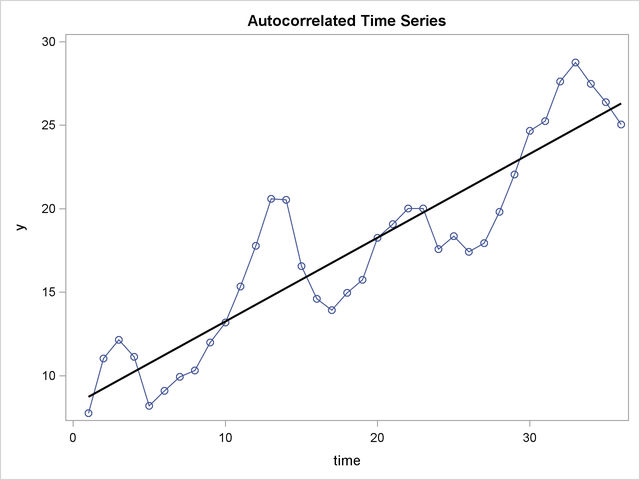
FIGURE 11.21: Autocorrelation

In a cross-sectional data-set, this assumption becomes one of saying no two observations $i$ and $j$ are correlated by design. I emphasize “by design” because in a genuine random sample, each unit has been selected into the sample independently of all other units and consequently this assumption should, in theory, be met. However, some units may end up being correlated for reasons unknown to us.

11.4.6 Assumptions 6, 7, and 8

Assumption 6 requires zero Covariance between $e$ and $x$. Formally, we need to have $E(e_i x_i = 0)$ and this is important because it allows us to reliably estimate the impact of a unit change in $x$ holding all else constant. If $E(e_i x_i \neq 0)$, then whenever $x$ changes, so does $e$. Think about this assumption as follows. In brief, the model we are fitting has been built by recognizing and measuring every independent variable known to influence $y$. If we have forgotten to include some variables that do influence $y$, these omitted variables will leak into the residuals (since the residuals represent all the variance of $y$ left unexplained by the model).

Assumption 7 requires that $n$ exceed the number of parameters to be estimated. Assume $n=2$, can you estimate $\hat{a}$ and $\hat{b}$? No you cannot because you will run into the degrees of freedom problem. So we always want to have a sufficiently large sample, and the more complex the regression model, the bigger the sample needed because each parameter that is estimated will use up a degree of freedom.

Assumption 8 requires variability in the $x$ values. Imagine if in a sample, all $x_i = x$. Now $\bar{x}=x$. What will happen to $SS_x$? It will be $0$, and no estimates will be calculable. Thus we require that the variance of $x$ be $> 0$. In other words, to calculate the effect of changes in $x$ on $y$, the sample values $x_i$ of must vary across observations in any given sample.

11.4.7 Assumptions 9 and 10

Assumption 9 requires that the model is correctly specified. Modeling always begins with theory, and by drawing a good sample, measuring the right variables correctly, and so on. Assume the TRUE MODEL is $y = a + b\left (\dfrac{1}{x} \right) + e$ but we don’t know this and estimate $y = a + bx + e$. Doing so will generate biased regression estimates! You can see this in the plot that follows, where for low values of $x$ we end up under-predicting $y$, then over-predicting $y$ in the middle-range of $x$ values, and again under-predicting $y$ for high $x$ values.

FIGURE 11.22: Model Misspecification

Of course, we rarely know the true model and hence it is all the more important that you have a sound theory to work with and the best data that you can gather to operationalize the theory.

Assumption 10 requires that there be no perfect Multicollinearity. This assumption comes into play when we go beyond a single $x$ variable to using multiple independent variables in a model such as $y = a + b_1x_1 + b_2x_2 + \ldots + b_kx_k + e$. In such an instance, multicollinearity implies that one or more of the $x$ variables are highly correlated. This becomes a problem because you cannot calculate the impact of a unit increase in $x_i$ by holding $x_j$ constant if $x_i$ and $x_j$ are highly correlated! There will always be some correlation between pairs of variables; that is not an issue. What is an issue is severe multicollinearity because it can increase the variance of the coefficient estimates and make the estimates very sensitive to minor changes in the model. The result is unstable regression coefficients that may even switch signs, making it difficult to specify the correct model. A classic sign of severe multicollinearity is when a model generates a high $R^2$ but very few of the independent variables are statistically significant. One way to minimize severe multicollinearity is to retain only one of a pair of highly correlated variables, combine them into some index via scaling techniques, or then try to increase the sample size since correlations tend to weaken in strength (not necessarily in statistical significance) with large samples.

There are several tests one could carry out to check for violations of these assumptions, and should some violations be discovered, there exist a vast array of techniques to adjust the model as well. Covering these techniques is beyond the scope of this introductory text but is addressed in the next text in this series. In that text we also extend the regression modeling framework to situations where the dependent variable is limited in some ways as, for example, a binary variable $(yes/no)$ or a count variable that measures the number of trips patients make in a year to the emergency room, the number of highway fatalities, and so on. We also cover regression techniques for panel data, and some interesting applications of regression discontinuity designs, propensity scores, mixed models, small area estimation techniques, sample selection models, and ordinal and multinomial models. For now, recognize the fact that two things are your best friend: (1) A good, substantive grasp of the factors that influence the dependent variable, and (2) access to a large random sample with accurate measurement of the independent and dependent variables. Without these bases covered, there is little value in fitting any sort of a statistical model.

11.5 Chapter 11 Practice Problems

Problem 1

Open up EPA’s Fuel Economy data. These data are the result of vehicle testing done at the Environmental Protection Agency’s National Vehicle and Fuel Emissions Laboratory in Ann Arbor, Michigan, and by vehicle manufacturers with oversight by EPA. Read the accompanying document available here to understand how some attribute is being measured.

fuelType1
charge120
cylinders
displ
drive
year
ghgScore
highway08
city08
model
trany
youSaveSpend

The data span several years so make sure you filter the file to retain only 2018 records. Now answer the following questions:

How are city miles per gallon (city08) correlated with highway miles per gallon (highway08)? Is the correlation significant?
Graph the relationship between these two variables.
As an intern at the EPA, your job is to determine if engine displacement (displ) has any impact on miles per gallon, and if it does, how much of an impact is it? Fit two regression models, one with city and the other with highway miles per gallon as the outcome of interest. Then, for each model,
1. Report and interpret the slope, the $\bar{R}^2$ and the standard error of the prediction.
2. Generate predicted values of miles per gallon both for the city and for the highway when displ = 1.5 versus when displ = 4.
3. Based on the two regressions you estimated, does a unit increase in displ have a larger impact on city miles per gallon or on highway miles per gallon?
Add the variable drive to both regression models. Now,
1. Report and interpret the impact of this new variable on miles per gallon
2. Evaluate whether the model fit has improved in terms of the $\bar{R}^2$ and the standard error of the prediction
3. Does drive have a larger impact on miles per gallon in the city or on the highway? What drive axle type has the largest versus smallest impact on city versus highway?

Problem 2

The next set of questions revolve around the 2016 Boston Marathon race results available here. The data-set contains the following variables:

Bib = the runner’s bib number
Name = the runner’s name
Age = the runner’s age (in years)
M/F = the runner’s gender (M = Male; F = Female)
City = the runner’s home city
State = the runner’s home state
Country = the runner’s home country
finishtime = the runner’s time (in seconds) to the finish line

Can we predict a runner’s finishing time on the basis of his/her age and gender? In order to answer this question,

Fit the appropriate regression model
Interpret the partial slopes, the $\bar{R}^2$ and the standard error of the prediction
Interpret the 95% confidence intervals around the partial slope of age
Draw a scatter-plot with the regression line superimposed along with the 95% confidence intervals
Based on your results, does it look like Age has a larger impact for a particular gender? Which one and what sort of an impact differential is there? (Hint: In order to answer this question you will need to suitably modify your regression model and review the results.)

Problem 3

Download the 2017 County Health Rankings data SPSS format from here, Excel format from here and the accompanying codebook. You should see the following measures (measurename)

Adult obesity
Children in poverty
High school graduation
Preventable hospital stays
Unemployment rate

Test for a pairwise correlation between all of these variables and note which ones are significant. Identify the pairs of variables that seem to be most strongly versus most weakly correlated with each other.

Problem 4

The data for this analysis come from the University of Michigan Panel Study of Income Dynamics (hereafter PSID) for the year 1975 (interview year 1976). Although this year was atypical of most of the 1970’s, only in 1976 did PSID directly interview the wives in the households. During all other years the head of the household’s interview supplied information about the wife’s labor market experiences during the previous year. One suspects that the own reporting is more accurate, and it is for this reason that many recent studies of married women’s labor supply have used these data.

This sample consists of 753 married white women between the ages of 30 and 60 in 1975, with 428 working at some time during the year. This sample size is smaller than most used in the studies reported in Table I. The dependent variable is hours = the wife’s annual hours of work in 1975, and measured as the product of the number of weeks the wife worked for money in 1975 and the average number of hours of work per week during the weeks she worked. The measure of the wage rate is the average hourly earnings, defined by dividing the total labor income of the wife in 1975 by the above measure of her hours of work.

inlf = labor force participation in 1975 = 1
hours = wife’s hours of work in 1975
kidslt6 = number of children less than 6 years old in household
kidsge6 = number of children between ages 6 and 18 in household
age = wife’s age
educ = wife’s educational attainment, in years
wage = wife’s average hourly earnings, in 1975 dollars
repwage = wife’s wage reported at the time of the 1976 interview (not= 1975 estimated wage)
hushrs = husband’s hours worked in 1975
husage = husband’s age
huseduc = husband’s educational attainment, in years
huswage = husband’s wage, in 1975 dollars
faminc = family income, in 1975 dollars
mtr = Federal marginal tax rate facing women
mothereduc = wife’s mother’s educational attainment, in years
fathereduc = wife’s father’s educational attainment, in years
unemprate = unemployment rate in county of residence, in percentage points
city = lives in large city (SMSA) = 1
exper = actual years of wife’s previous labor market experience
nwifeinc = $faminc - (wage \times hours)$ in thousand dollars
lwage = log(wage)
expersq = $exper^2$

The dependent variable of interest is wage, the wife’s average hourly earnings. Bearing this in mind,

Fit a regression model with the wife’s educational attainment as the independent variable. Interpret the partial slopes, as appropriate, and the fit of the model.
Now fit a regression model with the wife’s age, educational attainment, hours worked, and whether the household is in a large city or not.
Interpret the partial slopes, as appropriate, and the fit of the model.
Does adding the husband’s wage to the model improve the fit? Explain with reference to appropriate estimates from the revised model.

Problem 5

“The Student/Teacher Achievement Ratio (STAR) was a four-year longitudinal class-size study funded by the Tennessee General Assembly and conducted by the State Department of Education. Over 7,000 students in 79 schools were randomly assigned into one of three interventions: small class (13 to 17 students per teacher), regular class (22 to 25 students per teacher), and regular-with-aide class (22 to 25 students with a full-time teacher’s aide). Classroom teachers were also randomly assigned to the classes they would teach. The interventions were initiated as the students entered school in kindergarten and continued through third grade. The Project STAR public access data set contains data on test scores, treatment groups, and student and teacher characteristics for the four years of the experiment, from academic year 1985–1986 to academic year 1988–1989. The test score data analyzed in this chapter are the sum of the scores on the math and reading portion of the Stanford Achievement Test.” Source These data can be downloaded from here. Note the key variables as defined below:

gender = student’s gender
ethnicity = student’s ethnicity
stark, star1, star2, star3 = whether the student was in a small classroom, a regular classroom, or a regular classroom with a teaching aide
readk, read1, read2, read3 = reading test scores in kindergarten/grade 1/grade 2/grade 3
mathk, math1, math2, math3 = mathematics test scores in kindergarten/grade 1/grade 2/grade 3
lunchk, lunch1, lunch2, lunch3 = student eligible for free/reduced lunch in kindergarten/grade 1/grade 2/grade 3
schoolk, school1, school2, school3 = school type student attended in kindergarten/grade 1/grade 2/grade 3
degreek, degree1, degree2, degree3 = teacher’s highest degree earned in kindergarten/grade 1/grade 2/grade 3
ladderk, ladder1, ladder2, ladder3 = teacher’s career ladder status in kindergarten/grade 1/grade 2/grade 3
experiencek, experience1, experience2, experience3 = teacher’s years of teaching experience in kindergarten/grade 1/grade 2/grade 3
tethnicityk, tethnicity1, tethnicity2, tethnicity3 = teacher’s ethnicity in kindergarten/grade 1/grade 2/grade 3

Fit a regression model to predict a student’s third-grade reading score on the basis of his/her kindergarten score. Interpret the $\bar{R}^2$ and the standard error of the prediction, as well as the slope.
Fit a regression model to predict a student’s third-grade reading score on the basis of his/her kindergarten score, gender, ethnicity, and the type of classroom he/she was in during the third-grade.
Interpret, where appropriate, partial slopes
Interpret the $\bar{R}^2$ and the standard error of the prediction
Does adding information on the third-grade teacher’s years of experience improve the model fit? Explain.
What if you also added whether the student was eligible for free/reduced lunch? Does the fit improve? What, if anything, changes in the partial slopes?

Problem 6

The Ohio Department of Education gathers and releases a wealth of data on public schools and community schools; see, for instance, here and here. A snippet of these data are provided for you in this SPSS format file. An Excel version of the same data are available here Note that you have data for community schools and public school districts; private and parochial schools are excluded.

Check for correlations between the piscore (a measure used in the state’s accountability system with a higher score indicative of better performance), pctdisabled (percent of students attending the school who have a learning disability), pctecon (the percent of students who are deemed to be economically disadvantaged via measuring how many are eligible for free/reduced lunch), pctlep (the percent of students who have limited English proficiency), and pctminority (percent of students that are non-White). Report which correlations are/are not significant and the strength of these correlations as well.
Construct scatter-plots for all correlations tested above in part (a)
How well can you predict a school’s piscore? In order to answer this question, start by relying on the other variables listed in part (a) and folding them into the model as independent variables. Interpret all appropriate results, including the adjusted $R^2$ and the standard error of the prediction.
Does the prediction improve if you add school size (i.e., enrollment)? Note and report what changes and how.
What about if you add information on whether a school is a Community school (i.e., a charter school) or the traditional Public school? Note and report what changes and how.
All else being the same, does the model suggest that the average charter school performs better or worse than the average traditional public school? Explain.

Problem 7

These data reflect 392 observations on the following 9 variables.

mpg = miles per gallon
cylinders = Number of cylinders between 4 and 8
displacement = Engine displacement (cu. inches)
horsepower = Engine horsepower
weight = Vehicle weight (lbs.)
acceleration = Time to accelerate from 0 to 60 mph (sec.)
year = Model year
origin = Origin of car (1. American, 2. European, 3. Japanese)
name = Vehicle name

Note that the original data contained 408 observations but 16 observations with missing values have been removed.

Regress mpg on weight and interpret the slope, adjusted R-squared, and the standard error of the estimate.
Now estimate the following regression model: \[mpg = \alpha + \beta_1(cylinders) + \beta_2(acceleration) + \beta_3(weight) + \beta_4(origin) + \epsilon\] Be careful; some of the independent variables will have to be coded or even recoded given some problematic distributions and the fact that they are stored in the data-set as numeric but are in fact categorical variables.
Interpret partial slopes, where appropriate, as well as the model fit.
revise the previous model by adding an interaction between acceleration and manufacturing origin of the automobile. What estimates have changed and how? Has the fit improved or worsened? Interpret the interaction effects, if appropriate.
Visually represent the interaction effects, holding the number of cylinders at their modal value and weight at its median.
Use appropriate graphics to examine relationships between the variables you have in the regression model and see if anything seems to be amiss. For example, are distributions of weight, acceleration, mpg, and the number of cylinders roughly similar across manufacturing origin? Or do you see substantial differences?

Problem 8

These data are simulated data containing sales of child car seats at 400 different stores. The variables include

Sales = Unit sales (in thousands) at each location
CompPrice = Price charged by competitor at each location
Income = Community income level (in thousands of dollars)
Advertising = Local advertising budget for company at each location (in thousands of dollars)
Population = Population size in region (in thousands)
Price = Price company charges for car seats at each site
ShelveLoc = A factor with levels Bad, Good and Medium indicating the quality of the shelving loca- tion for the car seats at each site
Age = Average age of the local population
Education = Education level at each location
Urban = A factor with levels No and Yes to indicate whether the store is in an urban or rural location
US = A factor with levels No and Yes to indicate whether the store is in the US or not

The outcome of interest is the number of car seats sold (Sales) and the task given to you, as the chief data analyst for one of the largest retailers in the country is to figure out what features seem to best predict sales. Demonstrate your ability by fitting appropriate regression models and presenting the model that appears to perform the best.

Problem 9

These data reflect statistics for a large number of US Colleges from the 1995 issue of US News and World Report. The variables include

Apps Number of applications received
Private = A factor with levels No and Yes indicating private or public university Apps Number of applications received
Accept = Number of applications accepted
Enroll = Number of new students enrolled
Top10perc = Pct. new students from top 10% of H.S. class
Top25perc = Pct. new students from top 25% of H.S. class
F.Undergrad = Number of fulltime undergraduates
P.Undergrad = Number of parttime undergraduates
Outstate = Out-of-state tuition
Room.Board = Room and board costs
Books = Estimated book costs
Personal = Estimated personal spending
PhD = Pct. of faculty with Ph.D.’s
Terminal = Pct. of faculty with terminal degree
S.F.Ratio = Student/faculty ratio
perc.alumni = Pct. alumni who donate
Expend = Instructional expenditure per student
Grad.Rate = Graduation rate

You work for the Admissions office at your undergraduate alma mater and believe that you can use these data to figure out how to increase the number of applications accepted (Accept) at your university/college.

Start by visually exploring the data. Note down any instances where you see high correlations or strange distributions (for example, very skewed or even sparse), if any of these features vary by private versus public, and so on.
Fit and interpret the results from a regression model with Apps as the dependent variable and two independent variables – Private and Accept.
Now add Room.Board, Grad.Rate and perc.alumni. Reinterpret this updated model and evaluate if this model has improved our ability to predict Apps.
Remove any variable(s) that you thought, based on your work in (a), could be problematic given the usual assumptions that underlie regression analysis. Reinterpret the resulting model and compare with the previous models you fit to the data. Is your model performing better? Briefly explain your conclusion.

Problem 10

These data reflect a simulated data-set containing information on ten thousand customers. The aim here is to predict how much balance an individual is likely to carry on their credit card. The variables are:

ID = Identification
Income = Income in $10,000’s
Limit = Credit limit
Rating = Credit rating
Cards = Number of credit cards
Age = Age in years
Education = Number of years of education
Gender = A factor with levels Male and Female
Student = A factor with levels No and Yes indicating whether the individual was a student
Married = A factor with levels No and Yes indicating whether the individual was married
Ethnicity = A factor with levels African American, Asian, and Caucasian indicating the individual’s ethnicity
Balance = Average credit card balance in dollars

Visually explore the variables in the data-set (excluding the ID variable) and briefly write-up what you see in the data. Note any distributions that are of special concern.
Now fit a regression model with Balance as the dependent variable and the following independent variables: Rating, Income, Gender, Student, __Married_ and Ethnicity. Interpret your results.
Now eliminate all independent variables that are not statistically significant at $\alpha = 0.05$ and look at your estimates. Has the model improved or worsened? In what ways, if any?

Problem 11

These data reflect wage and other data for a group of 3000 male workers in the Mid-Atlantic region.

year = Year that wage information was recorded
age = Age of worker
maritl = A factor with levels 1. Never Married 2. Married 3. Widowed 4. Divorced and 5. Separated indicating marital status
race = A factor with levels 1. White 2. Black 3. Asian and 4. Other indicating race
education = A factor with levels 1. < HS Grad 2. HS Grad 3. Some College 4. College Grad and 5. Advanced Degree indicating education level
region = Region of the country (mid-Atlantic only)
jobclass = A factor with levels 1. Industrial and 2. Information indicating type of job
health = A factor with levels 1. <=Good and 2. >=Very Good indicating health level of worker
health_ins = A factor with levels 1. Yes and 2. No indicating whether worker has health insurance
logwage = Log of workers wage
wage = Workers raw wage

Subset the data-set to the year 2003 and fit the following regression model:

\[wage = \alpha + \beta_1(education) + \beta_2(jobclass) + \beta_3(race) + \beta_4(age) + \epsilon\] (b) Interpret your regression results. (c) Subset the data to 2009 and generate predicted values of wage with the 2003 regression estimates you generated in (a) (d) Generate an interaction between age and education and refit the model you estimated in (a) to the 2003 data. Does the model fit improve or worsen? What estimates change and how?

Problem 12

These data are from the 1971 Census of Canada and reflect the following variables:

education = Average education of occupational incumbents, years, in 1971
income = Average income of incumbents, dollars, in 1971
women = Percentage of incumbents who are women
prestige = Pineo-Porter prestige score for occupation, from a social survey conducted in the mid-1960s
census = Canadian Census occupational code
type = Type of occupation. A factor with levels: bc, Blue Collar; prof, Professional, Managerial, and Technical; wc, White Collar

The goal is to see if we can predict an occupation’s prestige on the basis of specific independent variables.

Fit a simple regression model with a lone independent variable – type and interpret the estimates.
Now add women to the model and see how the estimates change, if at all
Now add income and education and interpret the new estimates
Check to see if income and education are highly correlated, as should be expected. If they are, and the correlation is significant, exclude one of these from the model fit in (c) and see how the results change. Has there been any significant reduction in predictive ability or a substantial rise in our average prediction error?

Problem 13

Here are Andrew Gelman’s data on the IQ scores of some children and, for each child, information about their mother:

kid_score = child’s IQ score
mom_hs = whether the mother has a high school degree (=1) or not (=0)
mom_iq = mother’s IQ score
mom_age = mother’s age, in years
mom_work = mother’s work history, coded as 1 = did not work in first three years of child’s life, 2 = worked in 2nd or 3rd year of child’s life; 3 = worked part-time in first year of child’s life, and; 4 = worked full-time in first year of child’s life

Fit a simple regression model of the child’s IQ score as a function of the mother’s IQ score and whether the mother has a high school degree (or not)
Is there a significant interaction between the mother’s IQ and whether the mother has a high school degree (or not)? Test in a regression setting and state your conclusion.
Can you improve the model by adding the mother’s work history? Be sure to test for possible interactions, as appropriate and defensible.

Problem 14

These data come from the Institute for Democracy and Electoral Assistance (IDEA) and contain country-level information on voter turnout. Read all about the variables in this particular database here. I have added other variables, including Income Group that slots each country into the current World Bank classification system. The data-set thus includes the following variables:

Country = country name
Region = World region
Income group = World Bank classification
Year = Year turnout data refer to
Compulsory voting = whether voting is compusive or not, codes as “Yes” or “No”
turnout = Voter turnout (in percent)
vapturnout = Voting age population turnout (in percent)
popn = Population
vappopn = Voting age population
regdvoters = Number of registered voters
civilliberties = Freedom House’s rating on civil liberties (low = bad; high = good)
politicalrights = Freedom House’s rating on political rights (low = bad; high = good)

Fit a regression model with turnout as the dependent variable and popn as the independent variable. Interpret the results, including the model fit.
Now add whether voting is compulsory or not. How do the estimates change? How good is the model fit?
What if you add civilliberties and politicalrights? How do the results and the model fit change?
Add yet another variable, Income group. How do the results and the model fit change?
Given all the models you have fit, which model has the best overall fit? Focus on $\bar{R}^2$ and on the average prediction error.

Data Analysis for Leadership & Public Affairs: