Chapter 7 The Theory of Sampling Distributions

Every time that we draw a sample, we hope that it does indeed reflect the population from which it was drawn. But how much faith can we place in this hope? As it turns out, quite a fair amount of faith so long as we haven’t violated key tenets of sampling, have a sufficiently large sample to work with, and understand key elements of the theory of sampling distributions. That is our holy grail so let us not dither a second.

We can start by understanding two key elements of sampling, the science of drawing samples. One could draw samples in many different ways, several more complicated than others but at the heart of it all is our not violating two principles:

Each and every observation in the population has the same chance of being drawn into the sample
Each observation is drawn into the sample independently of all other observations

For example, if sampling from applicants to a job-training program at the welfare center, perhaps to see if a specific job-training program works (or not), I shouldn’t select applicants who seem to be younger or more engaged or non-Hispanic Whites, and so on because this would mean anybody who did not meet the selection criterion would have a $0$ probability of being sampled. Similarly, it would be a bad idea to select individuals who are obviously familiar with each other, maybe even related; by selecting one of them the chance of selecting another individual with them is far greater now than it would be if I didn’t know they knew each other, were related, etc. Samples that meet criteria (1) and (2) are referred to as simple random samples.

We also draw a distinction between finite populations (where we know the population size) and infinite populations (where we do not know the population size).

Finite Population: Draw a sample of size $n$ from the population such that each possible sample of size $n$ has an identical probability of selection
- We may sample with replacement, or
- sample without replacement (the more common – but not necessarily accurate – approach)
Infinite Population: We sample such that
- Each element is selected independently of all other elements
- Each element has the same probability of being selected

Now, assume we do this, that we draw all possible samples of a fixed sample size from a population. I’ll keep this simple by assuming the population is made up of only four numbers: 2, 4, 6, and 8. The population size, $N$ is $4$ and the population mean is $\mu = \dfrac{20}{4} = 5$. Now, what if I drew all possible samples of exactly $2$ numbers from this population and then calculated the sample mean $\bar{x}$ in each of these samples of $n = 2$? The result is shown below:

TABLE 7.1: An Example of Sampling Distributions
Sample No.	x1	x2	Mean
1	2	2	2
2	2	4	3
3	2	6	4
4	2	8	5
5	4	2	3
6	4	4	4
7	4	6	5
8	4	8	6
9	6	2	4
10	6	4	5
11	6	6	6
12	6	8	7
13	8	2	5
14	8	4	6
15	8	6	7
16	8	8	8

Eyeball the sample means in the column title $\bar{x}$ and you will see that the most commonly occurring sample mean is $\bar{x}=5$, which is equal to the population mean $\mu = 5$. Is this luck? Not at all. This is what the theory of sampling distributions tell us: On average, the sample mean will equal the population mean so long as the tenets of random sampling have not been violated. Formally, we state this as the Sampling Distribution of $\bar{x}$ is the probability distribution of all possible values of the sample mean $\bar{x}$. The Expected Value of $\bar{x}$ is $E(\bar{x})=\mu$ and the Standard Deviation of $\bar{x}$ is the Standard Error of $\bar{x}$, calculated for (a) Finite Populations as $\sigma_{\bar{x}}=\sqrt{\dfrac{N-n}{N-1}}\left(\dfrac{\sigma}{\sqrt{n}}\right)$ and for (b) Infinite Populations as $\sigma_{\bar{x}}=\dfrac{\sigma}{\sqrt{n}}$

Now, it should be somewhat intuitive that the larger the sample that we draw, the more likely is the sample mean to mirror the population mean. Is this true? Let us see with respect to the length of the human genome, something we have mapped almost completely, to the extent that we can deem it a known population. One way of seeing this in action is by first looking at the distribution of gene lengths (measured in nucleotides, “the sub-units that are linked to form the nucleic acids ribonucleic acid (RNA) and deoxyribonucleic acid (DNA), which serve as the cell’s storehouse of genetic information”). The population is shown below:

FIGURE 7.1: Population Distribution of Human Gene Lengths

The population mean human gene length is 2,622.027 and the standard deviation is 2,036.967. What would the distribution of sample means be if I drew 100 possible samples of $n=100$ from this population? What if I drew 100 samples with $n=1,000$, $n=10,000$, $n=15,000$? What if I drew all possible samples of $n=100$, $n=1,000$, $n=10,000$, $n=15,000$, calculated the mean in each sample and plotted the distribution of these means? What would such a distribution look like? Would most sample means cluster around the population mean or would they be wandering off, all over the place? Let us see these distributions mapped out for us. Note that the white vertical line in the plots that follows marks the population mean human gene length $(\mu = 2,622.07)$.

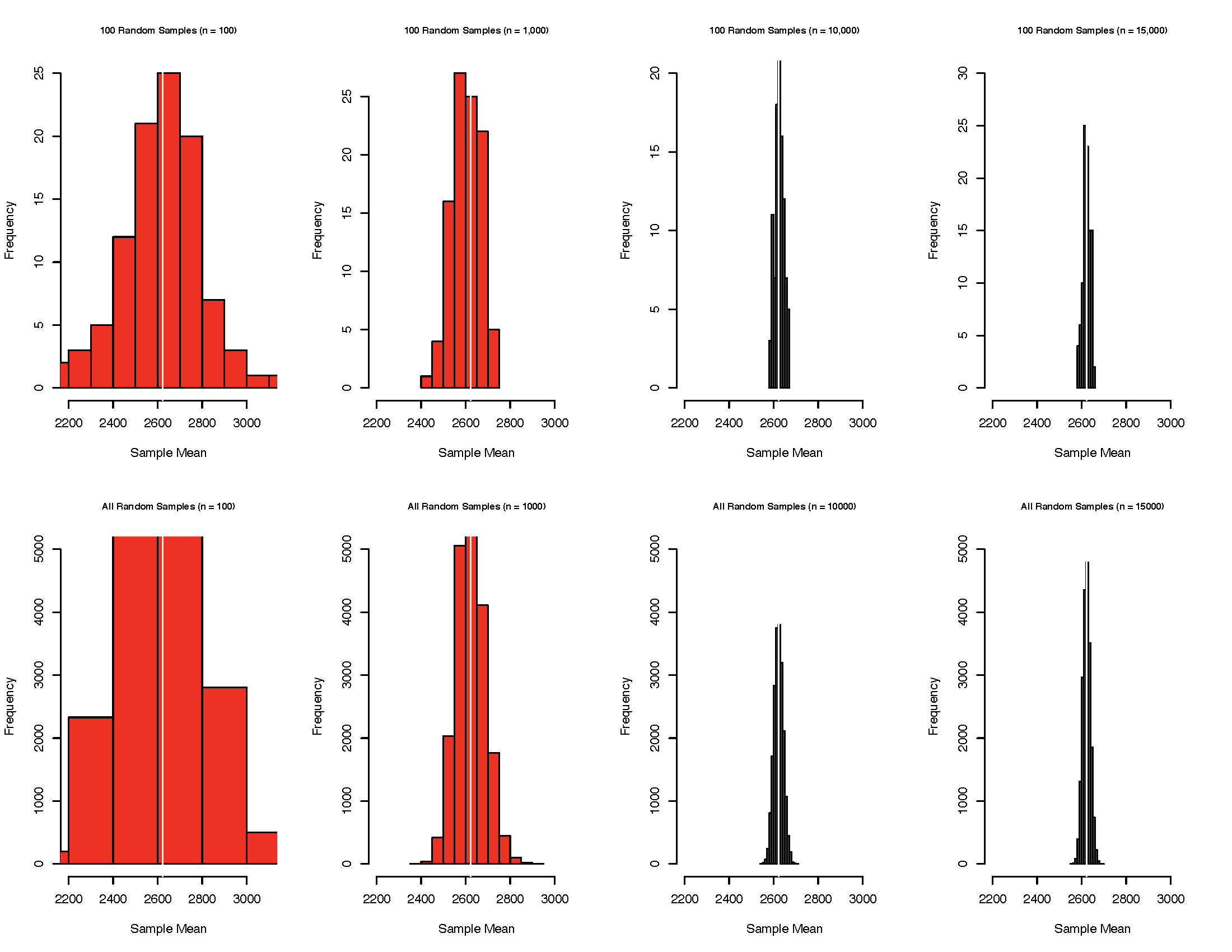
FIGURE 7.2: Sampling Distributions of Human Gene Lengths

Several noteworthy things are going on in these plots. First, individual sample means could end up anywhere in the distribution – some close to $\mu$ and some far away from $\mu$. Second, the larger the sample size, the more it seems that the resulting sample means tend to cluster around $\mu$. These two realizations should nudge you to wonder if sample size is the key to minimizing drift between your sample mean $\bar{x}$ and the population mean $\mu$. Yes, it is the key.

7.1 The Standard Error

If an important element of doing reliable data analysis is to have our sample mean be as close as possible to the population mean, is there a measure of how far our sample mean might be from the population mean? Yes there is, and we call it the standard error, denoted by $\sigma_{\bar{x}}$, where $\sigma_{\bar{x}} = \dfrac{\sigma}{\sqrt{n}}$. What does the standard error really tell us? Let us break its message down piece by piece.

First, you don’t see the population and so you have to rely on your sample mean to guess what the population mean might be. As such, one could say that the expected value of the sample mean is the population mean, i.e., $E(\bar{x}) = \mu$.
Now, if you were so lucky as to end up with a sample mean that is $\neq \mu$, how far away from $\mu$ do you think you might be? The answer is provided by the standard error, $\sigma_{\bar{x}}$. It is telling you the average distance of a sample mean from the population mean for all samples of a given sample size drawn from a common population with standard deviation of $\sigma$.

So clearly two things dictate how small or large the standard error could be – (i) how much variability there is in the population, i.e., the standard error $(\sigma_{\bar{x}})$, and (ii) how large a sample we are drawing, i.e., $(n)$. It should be very obvious that while we cannot influence variability in the population, sample size is under our control. Since $n$ figures in the denominator in the formula $\sigma_{\bar{x}} = \dfrac{\sigma}{\sqrt{n}}$, the larger is $n$, the smaller will $\sigma_{\bar{x}}$.

To recap, as $n \rightarrow \infty$, $\sigma_{\bar{x}} \rightarrow 0$ … that is, as the sample size $(n)$ increases the standard error $(\sigma_{\bar{x}})$ decreases …

\[\sigma=4000; n=30; \sigma_{\bar{x}}=\dfrac{\sigma}{\sqrt{n}}=\dfrac{4000}{\sqrt{30}}=730.2967\]

\[\sigma=4000; n=300; \sigma_{\bar{x}}=\dfrac{\sigma}{\sqrt{n}}=\dfrac{4000}{\sqrt{300}}=230.9401\]

\[\sigma=4000; n=3000; \sigma_{\bar{x}}=\dfrac{\sigma}{\sqrt{n}}=\dfrac{4000}{\sqrt{3000}}=73.0296\]

and, as $\sigma \rightarrow \infty$, $\sigma_{\bar{x}} \rightarrow \infty$ … that is, holding the sample size $(n)$ constant, samples drawn from populations with larger standard deviations $(\sigma)$ will have larger standard errors $(\sigma_{\bar{x}})$

\[\sigma=40; n=30; \sigma_{\bar{x}}=\dfrac{\sigma}{\sqrt{n}}=\dfrac{40}{\sqrt{30}}=7.3029\]

\[\sigma=400; n=30; \sigma_{\bar{x}}=\dfrac{\sigma}{\sqrt{n}}=\dfrac{400}{\sqrt{30}}=73.0296\]

\[\sigma=4000; n=30; \sigma_{\bar{x}}=\dfrac{\sigma}{\sqrt{n}}=\dfrac{4000}{\sqrt{30}}=730.2967\]

7.2 The Central Limit Theorem

But is this claim, of the sample mean $= \mu$ and if it isn’t, drifting, on average, by $\sigma_{\bar{x}}$ true for all population distributions? Yes, it is, by virtue of the Central Limit Theorem which stipulates that “For any population with mean $\mu$ and standard deviation $\sigma$, the distribution of sample means for samples of size $n$ will approach the normal distribution with a mean of $\mu$ and standard error of $\sigma_{\bar{x}}=\dfrac{\sigma}{\sqrt{n}}$ as $n \rightarrow \infty$.” This holds true so long as (i) the population is normally distributed, or (ii) the sample size is $\geq 30$ (note no reference is being made to the population being normally distributed). This is a very crucial theorem in statistics because it allows us to proceed with statistical analyses even when we cannot see the population (the default situation we almost always find ourselves in) so long as $n \geq 30$.

7.3 Applying the Standard Error and the Central Limit Theorem

7.3.1 Example 1

Tuition costs at state universities is $\sim \mu=\$4260; \sigma=\$900$. Sample of $n=50$ is drawn at random.

What is the sampling distribution of mean tuition costs?

\[\sigma_{\bar{x}}=\dfrac{\sigma}{\sqrt{n}}=\dfrac{900}{\sqrt{50}}= 127.28\]

What is $P(\bar{x})$ within $250 of $\mu$?

Sampling distribution is $\mu = 4260; \sigma_{\bar{x}} = 127.28$. Within $250$ implies $P(4010 \leq \mu \leq 4510)$

\[z_{4510}=\dfrac{4510-4260}{127.28}=1.96\]

\[z_{4010} = \dfrac{4010-4260}{127.28} = - 1.96\]

\[P(4010 \leq \mu \leq 4510) = 0.95\]

What is $P(\bar{x})$ within $100 of $\mu$? We want $P(4160 \leq \mu \leq 4360)$

\[z_{4360}=\dfrac{4360-4260}{127.28}=0.79\]

\[z_{4160} = \dfrac{4160-4260}{127.28} = - 0.79\]

\[P(4160 \leq \mu \leq 4360) = 0.5704\]

7.3.2 Example 2

Average annual cost of automobile insurance is $\sim \mu=\$687; \sigma=\$230$ and $n= 45$. Therefore, $\sigma_{\bar{x}}=\dfrac{\sigma}{\sqrt{n}}=\dfrac{230}{\sqrt{45}}= 34.29$. So the sampling distribution is $\mu = 687; \sigma_{\bar{x}} = 34.29$

What is $P(\bar{x})$ within $\$100$? We need $P(587 \leq \mu \leq 787)$

\[z_{787}=\dfrac{787-687}{34.29}=2.92\]

\[z_{587} = \dfrac{587-687}{34.29} = -2.92\] \[P(587 \leq \mu \leq 787) = 0.9964\]

What is $P(\bar{x})$ within $\$25$? We need $P(662 \leq \mu \leq 712)$

\[z_{712}=\dfrac{712-687}{34.29}=0.73\]

\[z_{662} = \dfrac{662-687}{34.29} = -0.73\]

\[P(662 \leq \mu \leq 712) = 0.5346\]

If insurance agency wants to be within $25, would you recommend a larger sample? Yes, since $n = 45$ is unlikely to yield the desired result.

7.4 The Sampling Distribution of Binary Proportions

The theory of sampling distributions also extends to binomial random variables. For example, assume that leadership training is sought and completed by some public agency personnel, mid-level perhaps. If we wanted to evaluate what proportion of mid-level public agency personnel have leadership training, we could draw a random sample. Let us assume that in the population, the proportion with such training happens to be $0.20$. Let us generate a sequence of 1,000,000 randomly drawn samples, first with $n=20$, then with $n=40$, and finally with $n=100$. The plots below show you the average proportion with leadership training. In each case, but most so in panels (b) and (c), we see what looks like a normal proportion. The takeway should be that in larger samples the proportion with leadership training is more likely to mirror the true proportion in the population, which turns out to be 0.20 (i.e., 20% of mid-level personnel have completed leadership training).

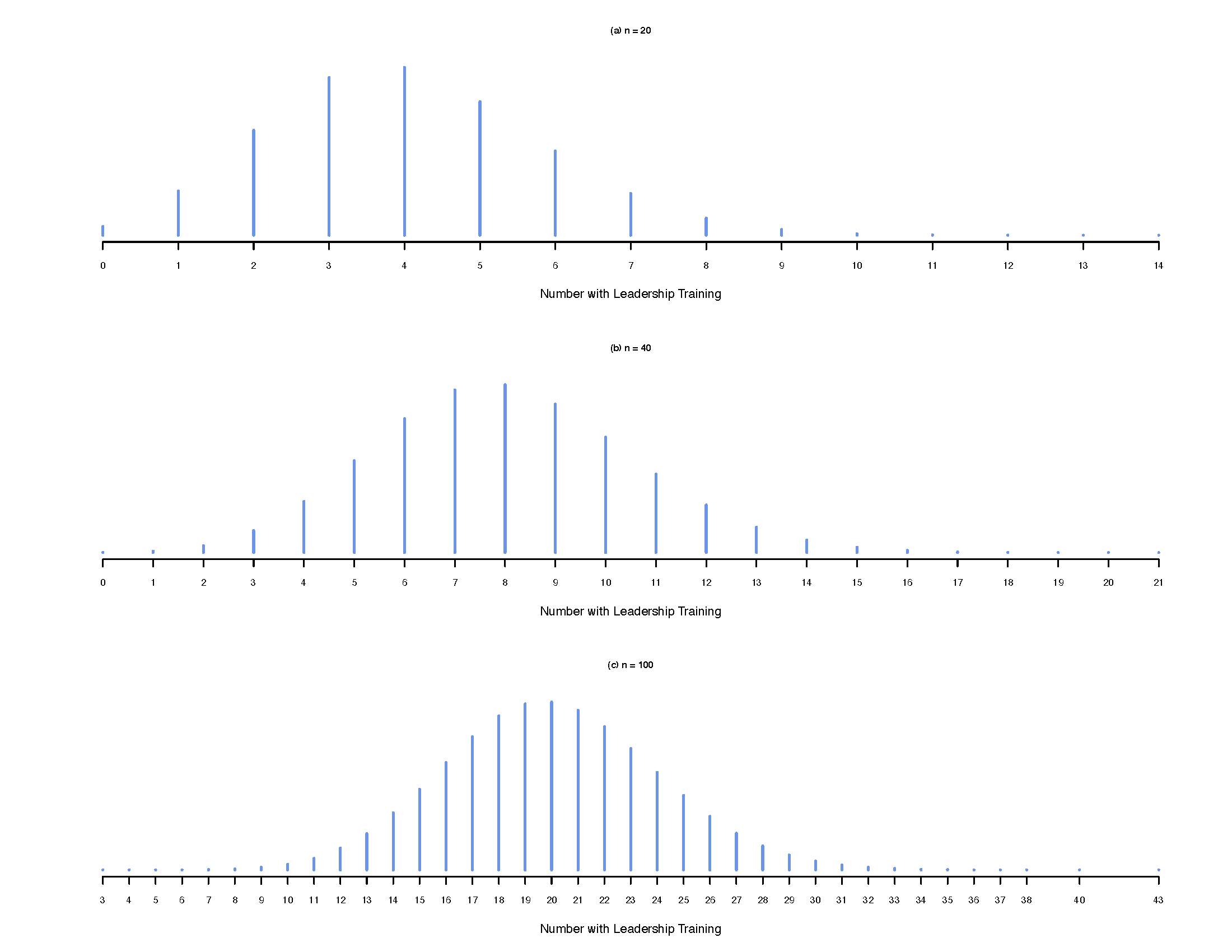
FIGURE 7.3: Sampling Distributions of Proportions

In general, then, the theory of sampling distributions applies as well to proportions as it does to means of continuous variables. Before we move on, however, let us see how the standard error is calculated for proportion and a few other key points.

The sample proportion is denoted by $\bar{p}=\dfrac{x}{n}$ and we expect, on average, that the expected value of the sample proportion is the population proportion, i.e., $E(\bar{p})=p$.

The standard error (aka the standard deviation of $\bar{p}$) is calculated as $\sigma_{\bar{p}}={\sqrt{\dfrac{p(1-p)}{n}}}$, and we can safely assume that the sampling distribution of $\bar{p}$ is approximately normally distributed if $np \geq 5$ AND $n(1-p) \geq 5$ (both conditions must be met).⁹

Note: When the population proportion $p$ is unknown, the standard error is calculated as $s_{\bar{p}}={\sqrt{\dfrac{\bar{p}(1-\bar{p})}{n}}}$

7.4.1 Example 1

The Governor’s office reports 56% of US households have internet access. If $p=0.56$ and $n=300$, what is:

The sampling distribution of $\bar{p}$? Given $n=300; p=0.56$, $\sigma_{\bar{p}}={\sqrt{\dfrac{0.56(1-0.56)}{300}}}=0.0287$
What is $Probability (\bar{p})$ within $\pm 0.03$? We are looking for the interval $(0.53,0.59)$ and so we calculate:

\[z_{0.59}=\dfrac{0.59-0.56}{0.0287}=1.0452\] \[z_{0.53}=\dfrac{0.53-0.56}{0.0287}=-1.0452\]

and hence $P(0.53 \leq \bar{p} \leq 0.59)=0.7031$

Calculate (1) and (2) for $n=600$ and $n=1000$, respectively.

7.4.2 Example 2

The Federal Highway Administration says 76 percent of drivers read warning signs placed by the roadside. Let $p=0.76$ and $n=400$. What is:

The sampling distribution of $\bar{p}$? Given $n=400; p=0.76$, $\sigma_{\bar{p}} = {\sqrt{\dfrac{0.76(1-0.76)}{400}}} = 0.0214$
$\text{Probability}(\bar{p})$ within $\pm 0.03$? We need $(0.73,0.79)$ so we calculate $z_{0.73}=\dfrac{0.73-0.76}{0.0214} = -1.40$ and $z_{0.79}=\dfrac{0.79-0.76}{0.0214} = 1.40$, and hence $P(0.73 \leq \bar{p} \leq 0.79) = 0.8385$
Repeat (1) and (2) for a sample of $n=1600$

7.5 Point Estimates

Statistics calculated for a population are referred to as population parameters (for e.g., $\mu$; $\sigma^{2}$; $\sigma$). On the other hand, statistics calculated for a sample are referred to as sample statistics (for e.g., ${\bar{x}}$; $s^{2}$; $s$). Since populations are beyond our reach we rely on samples to calculate point estimates. A point estimator is a sample statistic that predicts (or estimates) the value of the corresponding population parameter as for, example, in the sample mean $\bar{x}$ predicting/estimating the population mean $\mu$, the sample proportion $\bar{p}$ predicting/estimating the population proportion $p$, and so on. Not all point estimators are created equal, however. In fact, desirable point estimators have the following properties:

The sampling distribution of the point estimator is unbiased – it is centered around the population parameter. An unbiased estimator would be, for example, one that gives us $E(\bar{x}) = \mu$. If $E(\bar{x}) - \mu \neq 0$, we would have bias. Think of this as a case where the weighing scale in my house is not well calibrated and always shows the weight to be 10 pounds more than it actually happens to be. A different scale might always show a lower weight by 7.5 pounds than the true weight. Both these weighing scales are biased, one upwards the other downwards.
The point estimator is efficient – it has the smallest possible variance. Why does efficiency matter? It matters because if the point estimator has large variance we know our standard error will be large (recall: the numerator would be large), and hence the point estimator could have greater drift from the true population parameter. Thus, when choosing a point estimator from the set of point estimators we could work with, we prefer the one that has minimum variance.
The point estimator is consistent – it tends towards the population parameter as the sample size increases. This is the result that with increasingly larger samples the point estimate will come increasingly closer to the population parameter.

The easiest way to understand bias and efficiency is via the following graphic authored by Sebastian Raschka:

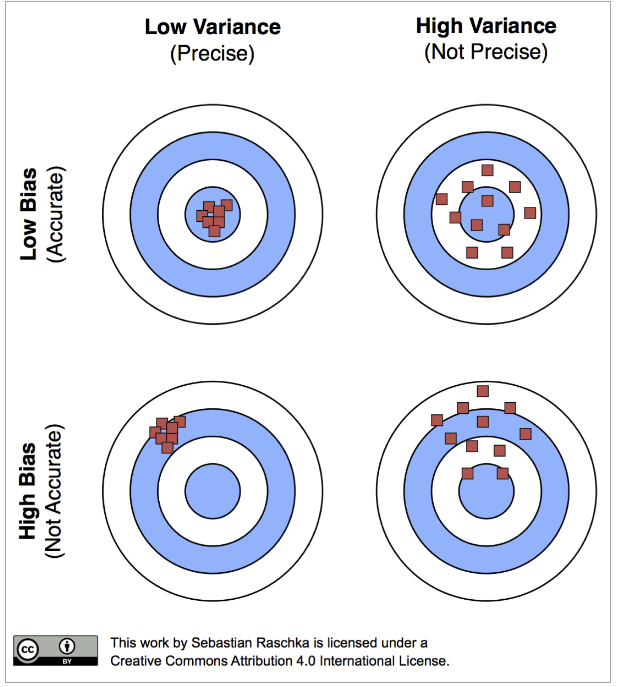
FIGURE 7.4: Bias and Efficiency of point estimates

The ideal point estimator has no bias and the smallest variance of all point estimators available to us, as shown by the red dots (each dot referencing a point estimate) in the top-left panel titled Low Bias (Accurate), Low variance (Precise). But a point estimate is by itself quite risky because it presents you with one possible value of the corresponding population parameter. For example, your sample might show median household income as $\bar{x} = 45,000$ and so you claim this is what the median household income must be for the population. However, if I asked you to bet a substantial amount of money on this estimate being accurate, you would (or should) not take the bet because there is a reasonable chance of you being wrong. Instead, if I asked you to give me a range of household income within which the population mean is likely to fall, now you have a span of values you could offer up with more confidence. This span of values is what we call interval estimates.

7.6 Interval Estimates

Although point estimates (for e.g., $\bar{x}$) tell us the expected value of a parameter based on a sample statistic, we know samples are not all the same even though they were drawn randomly, and have the same sample size. So we try to ask: How much confidence can we place in the point estimate? The margin of error helps us answer this question. Formally, the interval estimate of $\mu = \bar{x} \pm \text{ Margin of error}$ and the interval estimate of $p = \bar{p} \pm \text{ Margin of error}$ where the margin of error $= \left(z \times \sigma \right)$. In a base sense, what the margin of error is telling you is how far off, above or below the population mean or proportion, you should expect your sample mean or proportion to be. Hence the reference made in surveys to “The margin of error for this survey is $\pm 2.5$ percent,” and so on.

In any normal distribution of sample means with mean $\mu$ and standard deviation $\sigma$, the following statement is true: Over all samples of size $n$, the probability is $0.95$ for the event in question. That is, the distance between the sample mean and the population mean will fall in an interval covered by the margin of error: $-1.96\sigma \leq \bar{x}-\mu \leq +1.96\sigma$.

Rearranging the former identity yields: $\bar{x}-1.96\sigma \leq \mu \leq \bar{x} +1.96\sigma$. This expression says that in all possible samples of identical size $n$, there is a 95% probability that $\mu$ falls within a span of values given by $\bar{x} \pm 1.96\sigma$. The range of values within $\bar{x} \pm 1.96 \sigma$ yield the 95 percent confidence interval (CI) of $\mu$, and the two boundaries are the 95 percent confidence interval limits. Be careful! We aren’t saying $\mu$ falls within a known interval, although this is how most people treat confidence intervals. Rather, what we are saying is that in repeated random sampling if we drew all possible samples of a specific sample size $n$, calculated the 95 percent confidence interval in each sample, then plotted these confidence intervals, 95 percent of these 95 percent confidence intervals will include $\mu$. By extension, this also means that some 5 percent of these 95 percent confidence intervals will not include $\mu$. Watch the graph that follows; it shows you this principle in action.

In particular, the graph shows 100 confidence intervals as horizontal lines, with a vertical line demarcating the value of the population mean $(\mu = 20)$. Red horizontal lines are 95% confidence intervals that have completely missed the population mean.

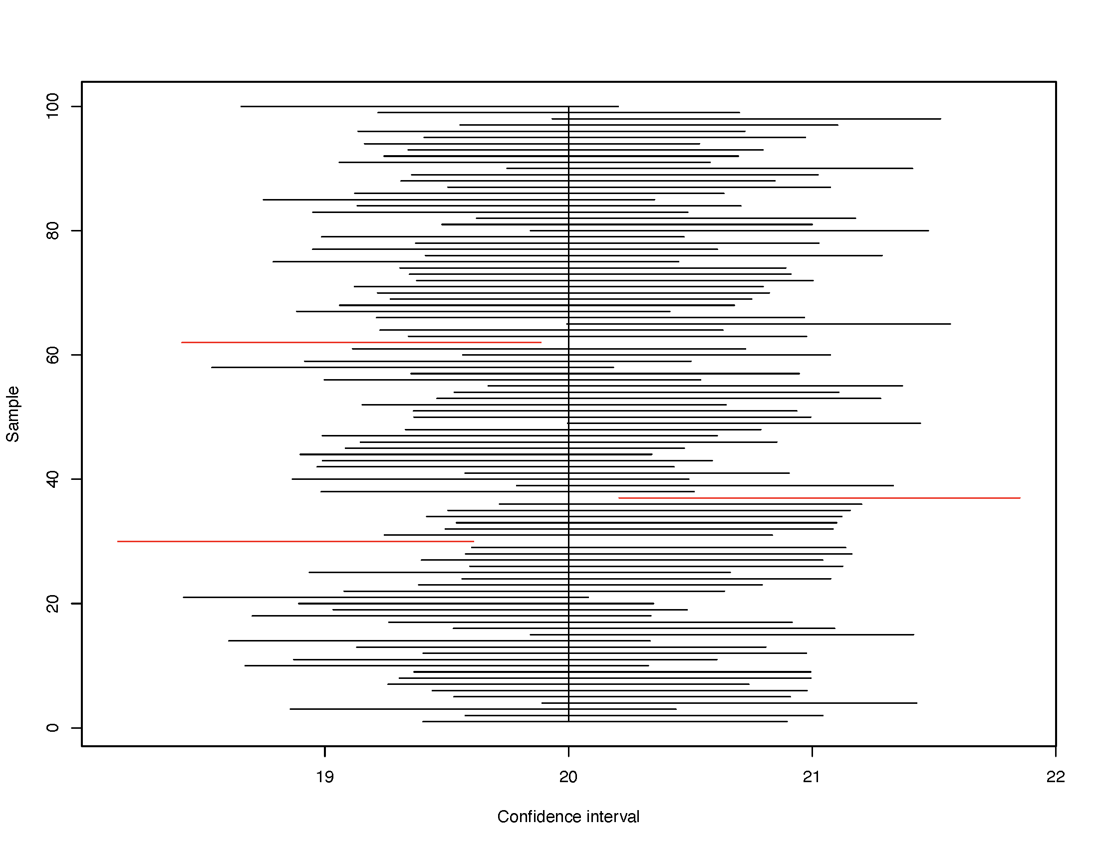
FIGURE 7.5: 95 Percent Confidence Intervals in 100 Random Samples

The second plot does the same thing anew by drawing 100 random samples and mapping the confidence intervals. This time around eight of these intervals miss the population mean.

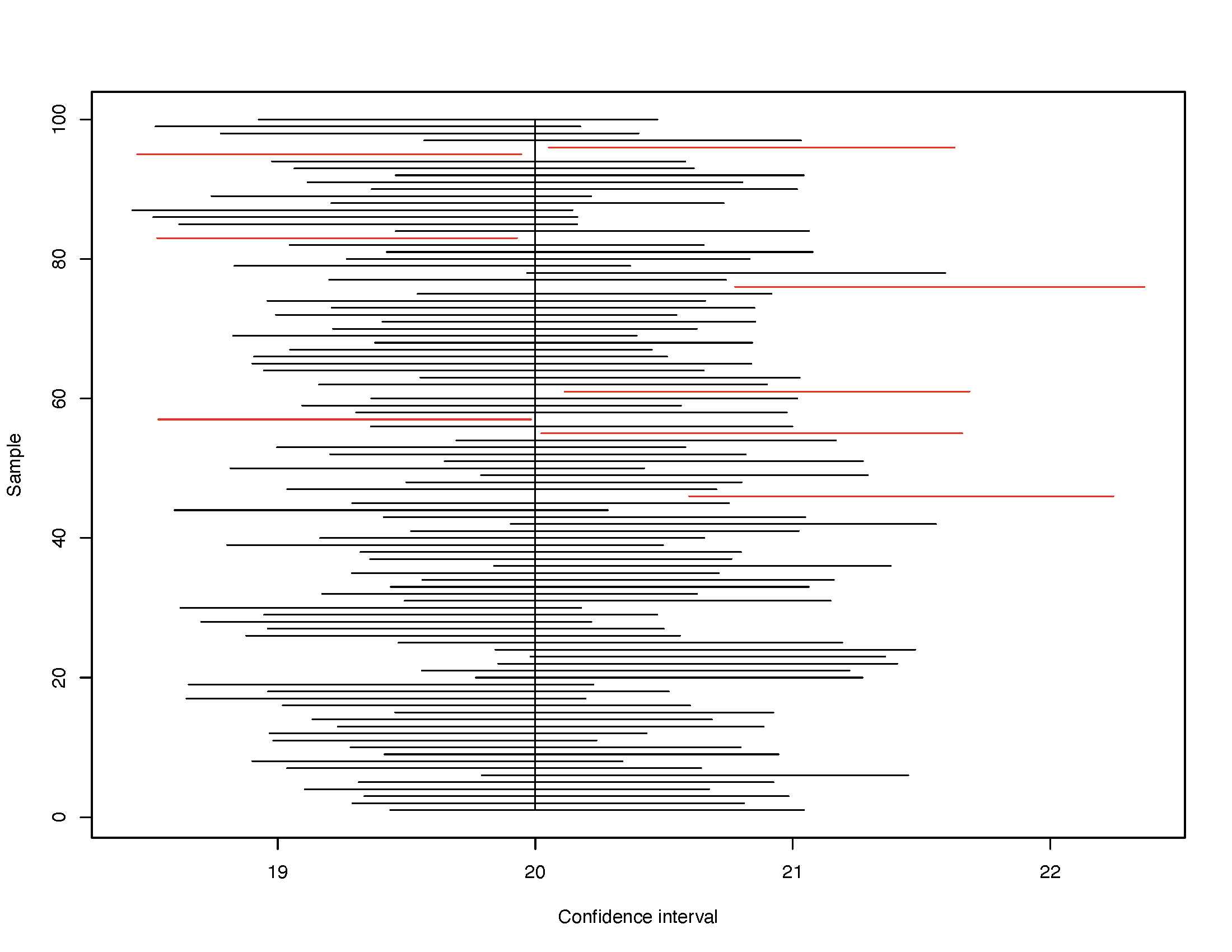
FIGURE 7.6: 95 Percent Confidence Intervals in 100 Random Samples

Before we move on to some examples, note the z-score values used in calculating the margin of error:

z = 1.645 for a 90% confidence level
z = 1.960 for a 95% confidence level
z = 2.576 for a 99% confidence level

7.6.1 Example 1

Let $\bar{x}=32; \sigma=6$. Let also $n=50$.

What is the standard error? $\sigma_{\bar{x}}=\dfrac{\sigma}{\sqrt{n}}=\dfrac{6}{\sqrt{50}}=0.8485$
Find $90\%$CI $= 32 \pm 1.645(0.8485)=32 \pm 1.3957=(30.6043; 33.3957)$
Find $95\%$CI $= 32 \pm 1.960(0.8485)=32 \pm 1.6630=(30.3370; 33.6630)$
Find $99\%$CI $= 32 \pm 2.576(0.8485)=32 \pm 2.1857=(29.8143; 34.1857)$

7.6.2 Example 2

Let household mean television viewing time be $\sim \bar{x}=8.5; \sigma=3.5$ and $n=300$. Therefore $\sigma_{\bar{x}}=\dfrac{\sigma}{\sqrt{n}}=\dfrac{3.5}{\sqrt{300}}=0.2020$

Find the $95$% CI $= 8.5 \pm 1.960(0.2020)=8.5 \pm 0.3959 = (8.1041; 8.8959)$
What is the $99$% CI? $= 8.5 \pm 2.576(0.2020) = 8.5 \pm 0.520352 = (7.979648; 9.020352)$

7.6.3 Interval Estimates for Binary Proportions

A similar logic applies to confidence intervals for binary proportions as well, with some differences in how the intervals are calculated. For one, since we don’t know the population proportion $p$ we calculate the standard error $s_{\bar{p}}$ as $s_{\bar{p}} = {\sqrt{\dfrac{\bar{p}(1-\bar{p})}{n}}}$. With the standard error in hand we could calculate a variety of confidence intervals but the three most often seen will be (i) the Agresti-Coull confidence intervals, (ii) the Wald confidence interval, and (iii) Wilson’s confidence intervals.

Agresti-Coull Confidence Intervals

The Agresti-Coull confidence interval requires us to first calculate $p^{'} = \dfrac{x + 2}{n + 4}$ and then calculate

\[p^{'} - z_{\alpha/2}\sqrt{ \dfrac{p^{'} \left(1-p^{'} \right) } {n+4} } \leq p \leq p^{'} + z _{\alpha/2}\sqrt{ \dfrac{p^{'} \left(1-p^{'} \right) } {n+4} }\]

Wald Confidence Intervals

Wald confidence intervals are calculated with the usual standard error and as:

\[\bar{p} - z_{\alpha/2}\sqrt{ \dfrac{\bar{p} \left(1-\bar{p} \right) } {n} } \leq p \leq \bar{p} + z_{\alpha/2}\sqrt{ \dfrac{\bar{p} \left(1-\bar{p} \right) } {n} }\]

These intervals are normal theory approximations and can be used as the default approach. However, they will yield very conservative intervals (i.e., confidence intervals that will be wider than they really should be) when (i) $n$ is small or (ii) $p$ is close to $0$ or $1$. In those cases you can rely upon the Agresti-Coull approach or, better yet, the Wilson approach (see below).

Wilson’s Confidence Interval

Wilson’s interval is calculated as follows:

\[\dfrac{n}{n + z^2_{\alpha/2}}\left[ \left(\bar{p} + \dfrac{z^2_{\alpha/2}}{2n} \right) \pm z_{\alpha/2} \sqrt{\dfrac{\bar{p}(1-\bar{p})}{n} + \dfrac{z^2_{\alpha/2}}{4n^2}} \right ]\]

which converts to

\[\dfrac{n}{n + z^2_{\alpha/2}}\left[ \left(\bar{p} + \dfrac{z^2_{\alpha/2}}{2n} \right) - z_{\alpha/2} \sqrt{\dfrac{\bar{p}(1-\bar{p})}{n} + \dfrac{z^2_{\alpha/2}}{4n^2}} \right ] \leq p \leq \dfrac{n}{n + z^2_{\alpha/2}}\left[ \left(\bar{p} + \dfrac{z^2_{\alpha/2}}{2n} \right) + z_{\alpha/2} \sqrt{\dfrac{\bar{p}(1-\bar{p})}{n} + \dfrac{z^2_{\alpha/2}}{4n^2}} \right ]\]

These are not the only intervals one could use and statistics software packages do not always use the same default approach. Hence it is always a good idea to check what method is being used by your software.

Before we move on to a few examples, note what happens at differing values of $\bar{p}$ for a given sample size.

TABLE 7.2: The Binomial Proportion Revisited
Proportion	1 - Proportion	(Proportion) * (1 - Proportion)
0.00	1.00	0.0000
0.05	0.95	0.0475
0.10	0.90	0.0900
0.15	0.85	0.1275
0.20	0.80	0.1600
0.25	0.75	0.1875
0.30	0.70	0.2100
0.35	0.65	0.2275
0.40	0.60	0.2400
0.45	0.55	0.2475
0.50	0.50	0.2500
0.55	0.45	0.2475
0.60	0.40	0.2400
0.65	0.35	0.2275
0.70	0.30	0.2100
0.75	0.25	0.1875
0.80	0.20	0.1600
0.85	0.15	0.1275
0.90	0.10	0.0900
0.95	0.05	0.0475
1.00	0.00	0.0000

Note what happens when $\bar{p}=0$ and $\bar{p}=1$: Your numerator in the formula $s_{\bar{p}} = \sqrt{\dfrac{\bar{p}(1-\bar{p})}{n}}$ is driven to $0$ and hence so is the standard error. So this problem occurs at the extremes of $\bar{p}$. Where the numerator $\bar{p}(1 - \bar{p})$ is the widest is when $\bar{p}=0.50$; as $\bar{p}$ moves away towards $0$ or $1$, $\bar{p}(1 - \bar{p})$ steadily decreases. At the extremes, the Wilson will do well but not so the Wald or Agresti-Coull

If you calculated the garden variety of confidence intervals for a case where $\bar{p} = 0.04166667$ you would see the following:

FIGURE 7.7: 95 percent Confidence Intervals when Sample Proportion = 0.0417

Note the variance in how wide the intervals are and that some of them cross $0$, which doesn’t make sense because you cannot have a negative sample proportion. On the other hand, if you calculated the garden variety of confidence intervals for a case where $\bar{p} = 0.5$ you would see muted differences between the different methods used to calculate confidence intervals (see below).

FIGURE 7.8: 95 percent Confidence Intervals when Sample Proportion = 0.5000

7.6.4 Example 1

In a survey of a small town in Vermont, voters were asked if they would support closing the local schools and sending the local kids to schools in the neighboring town to more efficiently utilize local tax dollars. A random sample of 153 voters yields 43.1% favoring school closures. What is the 95% confidence interval for the population proportion? Use the Wald approach.

We have $\bar{p}=0.431$ and $n = 153$. This yields a standard error of $s_{\bar{p}} = \sqrt{\dfrac{0.431(1-0.431)}{153}} = 0.04003585$.

Given $z = \pm 1.96$ the confidence interval is: $0.431 \pm 1.96(0.04003585) = 0.3525297 \text{ and } 0.5094703$. This can be loosely interpreted as: We are about 95% confident that the population proportion of the town’s voters that support school closures lies in the interval given by 0.3525 and 0.5094.

7.6.5 Example 2

Paper currency in the US often comes into contact with cocaine either directly or indirectly during drug deals or usage, or in counting machines where it wears off from one bill to the next. A forensic survey collected fifty $1 bills and traced cocaine on forty-six bills.

What is the best estimate of the proportion of US$1 bills that have detectable levels of cocaine?

The best estimate would be our sample proportion of $\bar{p} = \dfrac{46}{50} = 0.92$.

What is the 99% confidence interval for this estimate?

Since our sample proportion is close to $1$ we should use either the Wilson method or the Agresti-Coull approach. Here, the Wilson interval will be given by: 0.7657 and 0.9758. We can be about 99% certain that the proportion of US$1 bills with detectable levels of cocaine lies in the interval 0.7657 and 0.9758. The calculations are shown below:

\[\dfrac{n}{n + z^2_{\alpha/2}}\left[ \left(\bar{p} + \dfrac{z^2_{\alpha/2}}{2n} \right) - z_{\alpha/2} \sqrt{\dfrac{\bar{p}(1-\bar{p})}{n} + \dfrac{z^2_{\alpha/2}}{4n^2}} \right ]\] \[= \dfrac{50}{50 + 2.58^2}\left[ \left(0.92 + \dfrac{2.58^2}{100} \right) - 2.58 \sqrt{\dfrac{0.92(1-0.92)}{50} + \dfrac{2.58^2}{10000}} \right ]\]

and

\[= \dfrac{50}{50 + 2.58^2}\left[ \left(0.92 + \dfrac{2.58^2}{100} \right) + 2.58 \sqrt{\dfrac{0.92(1-0.92)}{50} + \dfrac{2.58^2}{10000}} \right ]\]

These are algebraically complex calculations and hence better done via a software package.

Note: There used to be a preference for the exact confidence interval (available in most software packages), and these are an interesting measure but the theory and algebra involved in calculating these intervals go beyond the scope of the class but you should be aware of them. You can use this online calculator for exact confidence intervals. These intervals will not be symmetric about the mean (i.e., extending the same distance above as they do below the mean). This is because a proportion cannot drop below $0$ or go beyond $1$. However, the intervals that use the normal approximation (like the Wald and the Agresti-Coull methods) do not recognize these constraints and hence fail when dealing with extreme sample proportions. However, of late consensus has veered in favor of the Wilson interval for small n and the Agresti-Coull for large n; see this article if you are interested in learning more about this guidance.

7.7 Student’s t distribution

In the preceding work with standard errors, margins of error, and confidence intervals we made a bold assumption – that we knew $\sigma$, variability in the population. However, if we don’t know $\mu$ and hence are trying to come up with the most precise estimate of $\mu$ via our sample $\bar{x}$, how can we really know $\sigma$? We cannot, and this is where Student's t distribution comes into play. This distribution was the brainchild of William Sealy Gosset, an employee of the Guinness Brewery. He worked with Karl Pearson on figuring out the challenges of using the standard normal distribution with small samples and unknown population variances. The distribution looks like the standard normal distribution but is fatter in the tails since in small samples more extreme results are possible. An applet is available here but let us see how this distribution works and why it matters.

Assume $X \sim N(13,2)$. If $x = 12, n=16$, what is $z_{x=12}$? It turns out that $z_{x=12}=2$. Now, what if we don’t know $\mu$ and $\sigma$ and draw three samples, each with $n=16$ but $s$ differs in each sample?

TABLE 7.3: The t distribution: An Example
Sample No.	Std. Dev.	Std. Error	z-score
1	4	1.00	-1
2	2	0.50	-2
3	1	0.25	-4

Notice what happens here: Each sample yields a different value of $z$ for the same $x=12$ simply because each sample is generating differing $\bar{x}$ and $s$. This leads to our making far more mistakes than we should if we continue to rely on the $z$ distribution. However, if you switch to the $t$ distribution we gain back some precision. The $t = \dfrac{x - \bar{x}}{s_{\bar{x}}}$ where $s_{\bar{x}} = \dfrac{s}{\sqrt{n}}$ and $t$ is distributed with $n-1$ degrees of freedom.

FIGURE 7.9: Student’s t versus the Standard Normal z Distribution

The red distribution is for the standard normal ($z$), and the blue distributions are for varying degrees of freedom, first for $df=1$ (panel (a)), then for $df=2$ (panel (b)), then for $df=3$ (panel (c)), and the black distribution is for $df=29$ (panel (d)). Notice that the distribution for $df=29$ is very close to the $z$ distribution. These plots illustrate the work of the $t$ distribution; for small samples, which then have smaller degrees of freedom, the $t$ deviates from the $z$ but as the $df$ increases, the $t$ starts mirroring the $z$ distribution. So is there a rule when you should use the $t$ instead of the $z$? Yes there is:

Use the $t$ distribution whenever $\sigma$ is unknown and hence the sample standard deviation $(s)$ must be used, regardless of the sample size
Use the $t$ distribution whenever $n < 30$ even if $\sigma$ is known

Note that disciplines vary in how they settle the question of when to use the $z$ versus the $t$. For example, some will use the $t$ whenever the sample size is less than 200 even if $\sigma$ is known while others will use $z$ whenever $\sigma$ is known regardless of the sample size. More prudent analysts will look for outliers and/or heavily skewed data, and if they see either of these issues, they may not rely on the $z$ unless the sample size is at least 50 or more (others would hold a higher standard, that of 100 or 200 data points). For our purposes, however, we will stick with the rule-of-thumb listed above for now.

7.7.1 Example 1

Find the following $t$ score(s):

$t$ leaves $0.025$ in the Upper Tail with $df=12$. Answer: $t=2.179$
$t$ leaves $0.05$ in the Lower Tail with $df=50$. Answer: $t=-1.676$
$t$ leaves $0.01$ in the Upper Tail with $df=30$. Answer: $t=2.457$
$90\%$ of the area falls between these $t$ values with $df = 25$. Answer: $t= \pm 1.708$
$95\%$ of the area falls between these $t$ values with $df = 45$. Answer: $t= \pm 2.014$

7.7.2 Example 2

Simple random sample with $n=54$ yielded $\bar{x} = 22.5$ and $s=4.4$.

Calculate the standard error. $s_{\bar{x}}=\dfrac{s}{\sqrt{n}}=\dfrac{4.4}{\sqrt{54}}=\dfrac{4.4}{7.34}=0.59$
What is the $90\%$ confidence interval? Answer: $\bar{x}\pm t(s_{\bar{x}})=22.5 \pm 1.674(0.59)=22.5 \pm 0.98=21.52; 23.48$
What is the $95\%$ confidence interval? Answer: $\bar{x}\pm t(s_{\bar{x}})=22.5 \pm 2.006(0.59)=22.5 \pm 1.18=21.32; 23.68$
What is the $99\%$ confidence interval? Answer: $\bar{x}\pm t(s_{\bar{x}})=22.5 \pm 2.672(0.59)=22.5 \pm 1.57=20.93; 24.07$
What happens to the margin of error and the width of the interval as we increase how “confident” we want to be? Answer: The margin of error increases and the confidence interval widens

7.7.3 Example 3

Pilots flying UN Peacekeeping missions fly, on average, 49 hours per month. This is based on a random sample with $n=100$ with $s=8.5$.

Find the margin of error for the 95% confidence interval. $s_{\bar{x}}=\dfrac{s}{\sqrt{n}}=\dfrac{8.5}{\sqrt{100}}=\dfrac{8.5}{10}=0.85$ and thus $t(s_{\bar{x}})=1.984(0.85)=1.68$
What is the $95\%$ confidence interval? $\bar{x}\pm t(s_{\bar{x}})=49 \pm 1.984(0.85)=49 \pm 1.68=47.32; 50.58$
How might we loosely interpret this interval? We might say that we can about 95% certain/confident that the population mean hours flown by pilots serving UN Peacekeeping missions falls in the interval given by $47.32$ hours and $50.58$ hours.

7.8 Key Concepts to Remember

If given $\sigma$ and $n \geq 30$, use the $z$
If given $\sigma$ and $n < 30$, use the $t$
If $\sigma$ is not provided and hence you have to use $s$, use the $t$ regardless of the sample size
Expected value of the sample mean is the population mean: $E(\bar{x}) = \mu$
Standard Error is $\sigma_{\bar{x}} = \dfrac{\sigma}{\sqrt{n}}$ when $\sigma$ is given and $s_{\bar{x}} = \dfrac{s}{\sqrt{n}}$ when $\sigma$ is unknown
Confidence Interval is given by $\bar{x} \pm z_{\alpha/2} \times \sigma_{\bar{x}}$ when using the $z$ and $\bar{x} \pm t_{\alpha/2} \times s_{\bar{x}}$ when using the $t$

7.9 Chapter 7 Practice Problems

Problem 1

Babies born in singleton births in the United States have birth weights (in kilograms) that are distributed normally with $\mu = 3.296; \sigma = 0.560$.

If you took a random sample of a 100 babies, what is the probability that their mean weight $\bar{x}$ would be greater than 3.5 kilograms?
If you took a random sample of a 25 babies, what is the probability that their mean weight $\bar{x}$ would be greater than 3.5 kilograms?

Problem 2

The most famous geyser in the world, Old Faithful in Yellowstone National Park, has a mean time between eruptions of 85 minutes. The interval of time between eruptions is normally distributed with a standard deviation of 21.25.

Suppose a simple random sample of 100 time intervals between eruptions was gathered. What is the probability that in this sample the mean eruption interval is longer than 95 minutes?
Suppose a simple random sample of 16 time intervals between eruptions was gathered. What is the probability that in this sample the mean eruption interval is shorter than 95 minutes?

Problem 3

The label on a one gallon jug of milk states that the volume of milk is 128 fluid ounces (fl.oz.) Federal law mandates that the jug must contain no less than the stated volume. The actual amount of milk in the jugs is normally distributed with mean $\mu = 129$ fl. Oz. and standard deviation $\sigma = 0.8$ fl. Oz.

Each shift, eight jugs of milk are randomly selected for thorough testing. The products are tested for filling volume, temperature, contamination, fat content, packaging defects, label placement, etc. Find the z-score corresponding to a sample mean volume (for these eight jugs) of 128 fl. Oz.
What is the probability that the sample mean of the volume for eight jugs is less than 128 fl. Oz.? (Give your answer accurate to 4 decimal places.)
What is the probability that the sample mean of the volume for eight jugs is greater than 128 fl. Oz.? (Give your answer accurate to 4 decimal places.)

Problem 4

In 2001 the average price of gasoline in the US was $1.46 per gallon, with a standard deviation of $0.15.

What is the probability that the mean price per gallon is within $0.03 of the population mean if you are working with a sample of 30 randomly selected gas stations?
What is the probability that the mean price per gallon is within $0.03 of the population mean if you are working with a sample of 50 randomly selected gas stations?
What is the probability that the mean price per gallon is within $0.03 of the population mean if you are working with a sample of 100 randomly selected gas stations?
Would you recommend a sample size of 30, 50, or 100 to have at least a 0.95 probability that the sample mean is within $0.03 of the population mean?

Problem 5

In a random sample of 120 students enrolled in graduate business degree programs, the average undergraduate grade point average (GPA) was found to 3.75. The population standard deviation is supposed to be 0.28.

What is the expected value of the average GPA of the population of students enrolled in graduate business degree programs?
What is the 95% confidence interval for this mean GPA?
What is the 99% confidence interval for this mean GPA?
What happens to the confidence interval as you move from (b) to (c)? Why? Briefly explain.

Problem 6

These data are records for a random sample of delayed flight arrivals on a single day at Chicago’s (IL) O’Hare Airport. Delays are reported in minutes.

Calculate the (i) mean, and the (ii) standard deviation of delays.
Calculate the standard error.
What is the expected value of the average delay for the population of all flights arriving at this airport?
What is the 95% confidence interval of average delay?
What is the 99% confidence interval of average delay?
If your sample size doubled, what would happen to the standard error?
If your sample size quadrupled, what would happen to the standard error?

Problem 7

If school absenteeism rate rises above 10% for a district, the state reduces its aid to the school district. Harpo Independent School District, a large urban district, draws a sample of five schools and find absenteeism rates to be 5.4%, 8.6%, 4.1%, 8.9%, and 7.8%, respectively.

What is your best estimate of the absenteeism rate in the school district?
What is the probability that the district’s absenteeism rate is more than 10%?
Find the 95% confidence interval for the district’s absenteeism rate.
How could you improve the precision of this confidence interval?

Problem 8

In 1955 John Wayne played Genghis Khan in The Conqueror, a movie shot (unfortunately) downwind of a site where 11 aboveground nuclear bomb tests were carried out. Of the cast and crew of 220 who worked on the movie, by the early 1980s some 91 had been diagnosed with cancer.

What is your best estimate of the population proportion of individuals exposed to these sites and diagnosed with cancer a little over two decades later?
What is the 95% confidence interval for this proportion?

Problem 9

A common perception is that individuals with chronic illnesses may be able to delay their deaths until after a special upcoming event, like a major holiday, a wedding, etc. Out of 12,028 deaths from cancer in a given year, 6052 occurred in the week before a special upcoming event.

What is the best estimate of the population proportion of deaths that occur in the week before a special upcoming event? What about in the week after a special event?
What are the respective 95% confidence intervals?

Problem 10

In a certain community with contaminated potable water supply, when pollsters asked a random sample of 232 residents if they would be willing to still use the water, 32 said “yes.”

Find the 95% confidence interval for the population proportion likely to say “yes.”
Find the 99% confidence interval for the population proportion likely to say “yes.”
Based on both confidence intervals, should the city make plans for alternative water delivery to residents because a majority of the population will not continue using the contaminated water? Explain.

Problem 11

In 1987, researchers studying the spread of AIDS collected data from a volunteer sample of 4955 adult males in Baltimore, Chicago, Los Angeles, and Pittsburgh. Of these men, 38% tested positive for AIDS.

What is the 95% confidence interval for the population proportion of adult males that might test positive for AIDS?
Since these data were gathered in a volunteer sample, they are clearly non-random. How might this impact your confidence interval? Explain.

Problem 12

Use the data provided here on motor vehicle occupant death rate, by age and gender, 2012 & 2014 to answer the questions that follow. Rate of deaths are calculated by age and gender (per 100,000 population) for motor vehicle occupants killed in crashes.

What is the best estimate of the population proportion of the death rate for all ages in your state in (i) 2012 versus (ii) 2014?
What is the 95% confidence interval for each estimate calculated above?

Technically, for a finite population, $\sigma_{\bar{p}}={\sqrt{\dfrac{N-n}{N-1}}}{\sqrt{\dfrac{p(1-p)}{n}}}$ and for an infinite population $\sigma_{\bar{p}}={\sqrt{\dfrac{p(1-p)}{n}}}$↩︎

Sample No.	x1	x2	Mean
1	2	2	2
2	2	4	3
3	2	6	4
4	2	8	5
5	4	2	3
6	4	4	4
7	4	6	5
8	4	8	6
9	6	2	4
10	6	4	5
11	6	6	6
12	6	8	7
13	8	2	5
14	8	4	6
15	8	6	7
16	8	8	8

Sample No.	x1	x2	Mean
1	2	2	2
2	2	4	3
3	2	6	4
4	2	8	5
5	4	2	3
6	4	4	4
7	4	6	5
8	4	8	6
9	6	2	4
10	6	4	5
11	6	6	6
12	6	8	7
13	8	2	5
14	8	4	6
15	8	6	7
16	8	8	8

Sample No.	x1	x2	Mean
1	2	2	2
2	2	4	3
3	2	6	4
4	2	8	5
5	4	2	3
6	4	4	4
7	4	6	5
8	4	8	6
9	6	2	4
10	6	4	5
11	6	6	6
12	6	8	7
13	8	2	5
14	8	4	6
15	8	6	7
16	8	8	8