Activity 1Install R program on your computer
1.1 Windows 10 users
1.1.1 Download and install R on your laptop at the link.
1.1.2 Click "start" at the left bottom corner on your screen
Type "R" in the "Type here to search"
If "R x64 4.0.2" is not shown under "All" dropdown menu, click "Apps"
Double click "R x64 4.0.2" to open R program.
1.2 Mac users
1.2.1 Download and install R on your laptop at the link.
1.2.2 Go to "/Applications/Utilities/" folder and find an application called "Terminal".
Double click to open "Terminal"
Type "R" to open R program in the Terminal.
1.3 Here is what you see in the R console
R version 4.0.2 (2020-06-22) -- "Taking Off Again"
Copyright (C) 2020 The R Foundation for Statistical Computing
Platform: x86_64-w64-mingw32/x64 (64-bit)
R is free software and comes with ABSOLUTELY NO WARRANTY.
You are welcome to redistribute it under certain conditions.
Type 'license()' or 'licence()' for distribution details.
Natural language support but running in an English locale
R is a collaborative project with many contributors.
Type 'contributors()' for more information and
'citation()' on how to cite R or R packages in publications.
Type 'demo()' for some demos, 'help()' for on-line help, or
'help.start()' for an HTML browser interface to help.
Type 'q()' to quit R.
>
Activity 2 Basic commands in R
The best way to learn programming is practicing. The two main components to handle in R programming are objects (variables)
and functions. Objects are variables, which can be assigned to anything that is saved in memory. Functions are actions that
R runs, such as creating a new object, making a graph (R is very powerful in graphing), reading a dataset, writing a file,
etc.
R creates objects using an assign operator, which is often a combination of a less than symbol and a hyphen, "<-". Sometimes,
an equal "=" symbol or "->" are also used.
From now on, you will become a R programmer. In the following instruction, there are two types of sentences. If the sentence(s)
is written beginning with a "#" or formatted with bold font, it provides an instruction or comment about what the R code works for. If the
sentence is written beginning with a ">", that is the real code you need to type into the R console. However, you only need to type the
content behind the ">" symbol since this symbol is automatically shown after you hit "enter" key when you finish the code. If a
sentence is italicised but not begins with a "#" nor a ">", that indicates the output of an R code you enter. Be
careful of the capital letters. In many cases, programming scripts are letter case sensitive.
2.1 Assign a variable
# We can create objects using the assign operator, "<-". For example, the following code creates a variable, "a", to which a value of 10 is assigned.>a<-10
# Since the value of a variable is temporally stored in the computer memory, we can see its output directly on screen by typing the
variable. For example, if you type "a" in R console, it will give an output “10” after you hit enter because the computer "remembers"
the value of 10 that has been assigned to "a".>a[1] 10
# "[1] 10" is the output. Once again, R scripts are case sensitive.>b<-10>B<-10000
# Check the output of "b" and "B".>b>B
2.2 Mathematical calculation
# If you don't have a calculator, R will be a good one for you. R can do all mathematical calculations that a calculator does.
Typing the following codes to see whether the output of each code is right.
>3+5
>(10 + 2) * 5
>2^2 # the square of 2
>sqrt(16) #square root of 16
>log(8,2) # log base 2 of 8
2.3 Use Functions
# You can create or directly apply functions from R libraries. The structure of an R function # is composed of a name followed by a
pair of round parentheses "()" that encircle the arguments taken by the function. Some functions do not require any arguments, such
as the "list" function, ls(), which lists all the objects in the current R session.
>name <-"Jacob"
>n1<-10
>n2<-100
>m<-0.5
>ls()
# The following output will be shown on screen after you finish entering ls(), which lists all the variables you have created by far in
your R session.
[1] "a" "b" "B" "m" "n1" "n2" "name"
Activity 3 Data objects (variables) in R
# There are five types of data objects in R: vector, factor, data matrix, data frame, and list. All data objects have attributes
and values. Due to learning scope, we only briefly introduce how to manipulate data frame, data matrix and barplot graphing
in this learning practice. If you wish to learn more, you may consider taking my PBIO 4280 - Laboratory in Genomics
Techniques (3 credits).
# A data frame in R can be created (assigned) by reading a spreadsheet file. Certainly, it can also be created by R functions. However,
barplot() function recognizes data matrix but not data frame for drawing a graph.
3.1 Download files
# We will use the sample of a spreadsheet file based on Table 1 of your Lab 3
Table 1. Number of cells under different mitosis stages.
---------------------------------------------------------------------------
|---------------|--Prophase--|--Metaphase--|--Anaphase----|--Telophase--|
---------------------------------------------------------------------------
|--Your_Data----|-----64-----|-------26-----|-------39------|------25-----|
---------------------------------------------------------------------------
|--Class_Data---|----1256----|-----839------|-------695-----|-----930----|
---------------------------------------------------------------------------
# We will use download.file() function to download the file directly in your R session. You may just copy and paste the code below
in your R console (do not copy the > symbol!). The basic argument of download.file() requires the URL address of a source file,
a destination file name
(destfile), and a method for downloading the file. Here the sources file is saved on my GitHub account at Source File. The name of the
destfile is "cell_number.csv". We use a method of auto to download the file
>URL<-"https://raw.githubusercontent.com/hua-lab/PBIO1140/master/data/Number_of_cells_w_different_mitosis_stages.csv"
>download.file(URL,destfile='cell_number.csv',method='auto')
# 3.2 Read CSV Files
# The file is originally written as a "comma-separated values" (csv) file. It can be read and opened in Excel. However, we will learn
R to read and assign it to a data frame object (variable), df1.
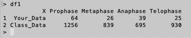
>df1<-read.csv(file="cell_number.csv",header=TRUE)
# We use read.csv() function to read in the file. Since the spreadsheet contains column names, which R also recognizes as "header",
we tell read.csv() that the file has a header by header=TRUE.
>df1
# You will see an output as follows.
Activity 4 Draw a graph in R
# R is very powerful in drawing beautiful and scientifically meaningful graphs. That is another important reason why I strongly recommend
you to learn. There are many great graphing packages in R. Here we use
a useful barplot() to draw a bar graph based on the data in Table 1.
4.1 Convert a data frame to a data matrix
# Before we draw the graph, we need to understand the structure of a data frame and learn how to convert it into a data matrix
that barplot() can recognize.
>df1[1,1]
[1] Your_Data
Levels: Class_Data Your_Data
# This code reads the value of the cell in Row 1 and Column 1.
>df1[2,1]
[1] Class_Data
Levels: Class_Data Your_Data
# This code reads the value of the cell in Row 2 and Column 1. You may recognze none of the values from Column 1 cells are numeric
>df1[1,2]
[1] 64
# This code reads the value of the cell in Row 1 and Column 2. This value is numeric.
# You may also notice that each cell in a data frame can be read by a combination of row number and column number. The two numbers are separated
by a comma and wrapped in a pair of brackets.
# We can also see the output does not have any numeric value for cells in column 1. Instead, it reads the names of our two datasets (Your_Data
and Class_Data) in Table 1.
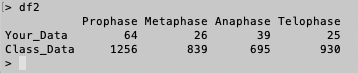
# We do some R coding to remove the "X" column, create rownames (not cells), and save the new data frame to a new object, df2.
>df2<-df1[,-1]
>df2
# Remove the first column of df1 and assign the new data frame to df2.
>rownames(df2)<-df1[,1]
>df2
# Assign the values in the first column of df1 as the rownames of df2.
>df2<- as.matrix(df2)
>df2
 >df1
>df1
# You can see the top of rownames in
df2 does not have any characters. However, there is an "X" character on top of the first column in
df1. Indeed, the row names of
df1 are "1" and "2", and the row names of
df2 are "Your_Data" and "Class_Data", which
are more meaningful.
> rownames(df1)
[1] "1" "2"
> rownames(df2)
[1] "Your_Data" "Class_Data"
4.2 Draw a barplot graph
# as.matrix() function in 4.1 converts a data frame into a data matrix so that batplot() function can use
the data matrix to make a bar graph.
>barplot(df2, beside=TRUE, legend.text = TRUE, col = c("red", "green"), args.legend = list(x = "topright", bty = "n", inset=c(-0.05, 0)),xlab="Mitosis Stages",ylab="Number of Cells",main="Number of Cells under Different Mitosis Stages")
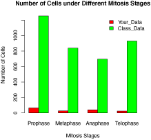 Figure 1. Comparison of cell population under different mitosis stages. The cells under each mitosis stage of a garlic root tip were counted based on the morphology of chromosomes stained with aceto-orcein. The red and green bars represent the data obtained from yours and the entire class, respectively.
4.3 Save a graph file
# If you don't see a graph pop-up, you can save the graph as a PDF file and open it with a PDF file reader. You may further edit and
incorporate it into your lab report.
>pdf("cell_number_comparison_mitosis.pdf",height=5,width=5)
>barplot(df2, beside=TRUE, legend.text = TRUE, col = c("red", "green"), args.legend = list(x = "topright", bty = "n", inset=c(-0.05, 0)),xlab="Mitosis Stages",ylab="Number of Cells",main="Number of Cells under Different Mitosis Stages")
>dev.off()
# dev.off() closes the graphing process.
# The PDF file, named "cell_number_comparison_mitosis.pdf", should be saved in your R working directory, which can be detected in R by the
function, getwd(). In my case, the file is saved at "/Volumes/macbook_d/Teaching/2020_Fall".
> getwd()
[1] "/Volumes/macbook_d/Teaching/2020_Fall"
# Use function quit("yes") to terminate you R session.
>quit("yes")